12. Pattern Graphs

Grokking Interview Pattern Interview

Word count: 8.6kReading time: 53 min

 2024/05/12 

Introduction to Graph

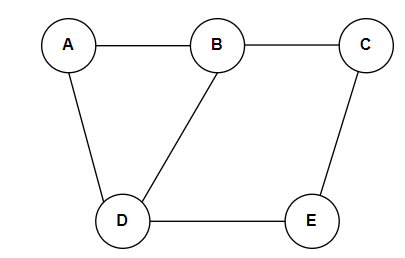
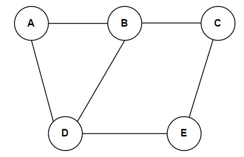
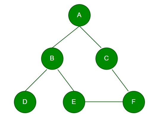
A graph is a data structure that consists of a set of vertices (nodes) and a bunch of edges connecting these vertices. Graphs are widely used to model real-world scenarios where relationships and connections between entities must be represented. A Graph G (V, E) with five vertices (A, B, C, D, E) and six edges ((A, B), (B, C), (C, E), (E, D), (D, B), (D, A)) are shown in the following figure.

Graphs can become more complex as they grow and have many interconnected nodes and edges. Graphs are a fundamental and versatile data structure used in various computer science applications to model and solve complex problems involving relationships and connections.

Application of Graphs

Graphs are versatile data structures that find applications in various fields. Here are five graph applications with facts and figures:

1. Social Network Analysis: Graphs are widely used for analyzing social networks to understand connections between individuals or entities. One of the most popular social networks is Facebook.

2. Transportation Network Optimization: Graphs are crucial in optimizing transportation networks like road or flight routes. For example, the road network of the United States spans over 4 million miles. Using graph algorithms like Dijkstra’s algorithm, authorities can efficiently find the shortest path between two locations, minimizing travel time and fuel consumption.

3. Internet and Webpage Ranking: Search engines like Google use graphs to rank webpages and determine their relevance to a search query. Google’s PageRank algorithm, which Larry Page and Sergey Brin introduced, utilizes a graph representation of the web.

4. Recommendation Systems: Graphs are employed in recommendation systems to provide personalized suggestions to users based on their preferences and behaviors. A popular streaming platform, Netflix uses a graph-based collaborative filtering approach to recommend movies and TV shows to its subscribers.

5. Bioinformatics and Protein Interactions: In bioinformatics, graphs model complex biological interactions, such as protein-protein interactions, gene regulatory networks, and metabolic pathways. The Human Protein Reference Database (HPRD), which stores protein-protein interaction data, contains information about more than 39,000 interactions among over 9,000 proteins.

These examples demonstrate the wide-ranging applications of graphs in different domains, each significantly impacting the respective industries.

Common Graph Terminologies

Understanding baseline graph terminologies is essential for understanding complex graph concepts. Like the other concepts, graph theory has some baseline terminologies. These terminologies are the most commonly used jargon in graphs. Understanding these jargons empower you better understand and communicate the graph concept.

Here are some of the most commonly used graph terminologies:

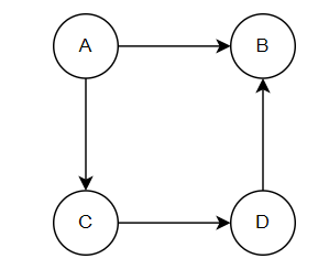
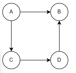
1. Digraph:

A digraph, short for directed graph, is a type of graph in which edges have a direction or are represented by arrows. Each edge connects two vertices (nodes), but the direction of the edge indicates a one-way relationship between the nodes. In other words, if there is an edge from vertex A to vertex B, you can only travel from A to B along that edge.

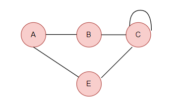
3. Loop in Graph:

A “loop” in a graph refers to an edge that connects a vertex to itself. In other words, it is an edge that starts and ends at the same vertex. Loops can exist in both directed and undirected graphs.

In an undirected graph, a loop is simply an edge that connects a vertex to itself. It forms a cycle of length 1. For example, if you have a graph with a single vertex v, and there is an edge from v to itself, then it forms a loop.

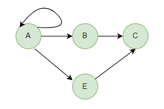
In a directed graph, a loop is an arc (directed edge) that starts and ends at the same vertex. It forms a directed cycle of length 1. For example, if you have a graph with a single vertex v, and there is a directed edge from v to itself, then it forms a loop.

4. Node in Graph:

A “node” (also known as a “vertex”) is a fundamental building block of a graph. A graph is a mathematical representation of a set of vertices (nodes) and the connections (edges) between those objects. The links between nodes can be either directed or undirected, depending on whether the relationship has a specific direction. In the following figure, A, B, C, D, and E are the nodes in the graph, also known as vertices.

5. Adjacent Nodes:

Two nodes are said to be adjacent if an edge is connected directly. The set of nodes adjacent to a particular node is known as its neighborhood. As in the above figure, the nodes A and B are adjacent.

6. Degree of a Node:

The degree of a node is the number of edges connected to it. In an undirected graph, it represents the number of neighbors a node has. As in the above figure, the degree of Node A is two because it has two neighbors.

In a directed graph, there are two degrees:

The in-degree (number of incoming edges)
The out-degree (number of outgoing edges).

In the above graph, the degree of node A is two because two edges are outgoing, and the degree of node C is 1.

7. Path:

A sequence of vertices in which each consecutive pair of vertices is connected by an edge. For example in the above figure, there is a path from vertex A to B.

8. Cycle:

A path in which the first and last vertices are the same, forming a closed loop. The following figure shows a route from A to B, B to D, D to C, and C to A. So here, the cycle completes because we start from vertex A and end again at A vertex.

Graph Types

There are several types of graphs, each with its specific characteristics. Here are some common types of graphs, along with examples:

1. Undirected Graph: In an undirected graph, edges have no direction, representing a bidirectional connection between two vertices. If an edge exists between vertex A and vertex B, you can traverse from A to B and vice versa.

Example: Friends Network

2. Directed Graph: In a directed graph, edges have a direction, indicating a one-way connection between vertices. If there is an edge from vertex A to vertex B, you can only traverse from A to B, not vice versa.

Example: Webpage Links

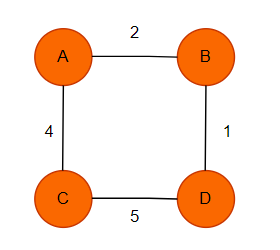
3. Weighted Graph: Each edge is associated with a numerical value called a weight in a weighted graph. The weight can represent distances, costs, or any other relevant metric between the connected vertices.

Example: Transportation Network

4. Unweighted Graph: All edges have the same default weight of 1 in an unweighted graph. There are no additional numerical values associated with the edges. In an unweighted graph, the absence of edge weights implies that all edges are considered to have equal importance or distance between the connected nodes.

Example: Family Tree (Connection exists or doesn’t)

5. Cyclic Graph: A cyclic graph is a graph that contains at least one cycle, which is a closed path (sequence of vertices) that starts and ends at the same vertex.

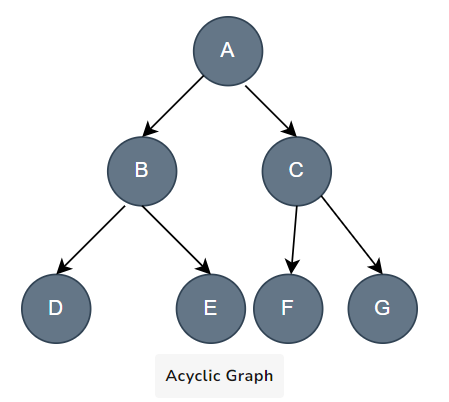
6. Acyclic Graph: An acyclic graph is a directed graph that has no cycles. A cycle occurs when the following edges from a node lead back to the same node. Some key properties of acyclic graphs:

They have at least one node with no incoming edges (called a source node).
They have at least one node with no outgoing edges (called a sink node).

In this graph, node A is the root node. It has no incoming edges. Nodes D, E, F, G are leaf nodes - they have no outgoing edges. There are no cycles in this graph.

A valid topological ordering of the nodes could be: A, B, C, D, E, F, G. So this graph structure forms an acyclic-directed graph. Trees and DAGs (Directed Acyclic Graphs) are common examples of acyclic graph structures

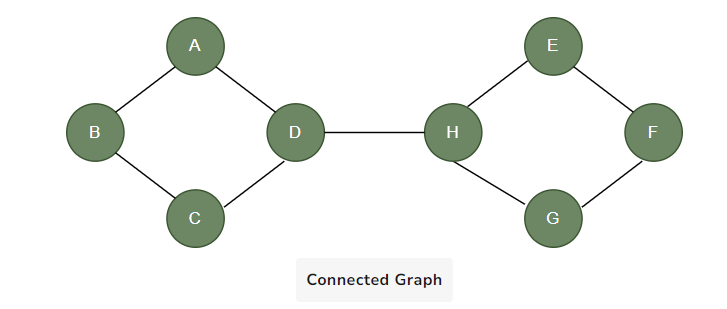
7. Connected Graph: A connected graph is one in which there is a path between every pair of vertices. In other words, every vertex is reachable from any other vertex in the graph.

8. Disconnected Graph: A disconnected graph has two or more connected components (subgraphs) with no direct connection between these components. The figure below is one separate graph. The first component contains A, B, C, and D vertices, and the other part contains E, F, G, and H, with at least two vertices not connected by a path.

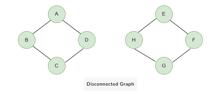
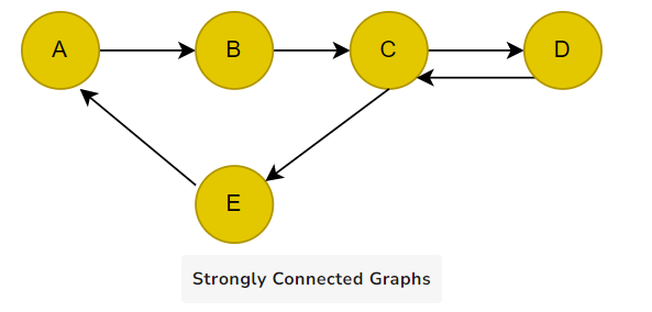
9. Strongly Connected Graphs: A strongly connected graph is a type of directed graph in which there is a directed path from every vertex to every other vertex. In other words, for any two vertices, A and B, in a strongly connected graph, there is a directed path from A to B and B to A.

These are some of the common types of graphs in data structures. Each type has its significance and use cases depending on the problem you’re trying to solve. Understanding different types of graphs is crucial for effectively applying graph algorithms and solving graph-related problems.

Graph Representations

We primarily represent graphs using two ways:

Adjacency matrix
Adjacency list

Let’s explore what they are.

Adjacency Matrix

An adjacency matrix is a common way to represent a graph as a matrix. It is a square matrix where the rows and columns represent the vertices of the graph, and the entries (elements) of the matrix indicate whether there is an edge between the corresponding vertices.

In an undirected graph, the edges have no direction, meaning they can be traversed in both directions between two vertices. On the other hand, in a directed graph, the edges have a direction, indicating a one-way relationship between two vertices.

As there are two major types of graphs directed graph and undirected graph. Let’s see how the adjacency matrix works for both types of graphs:

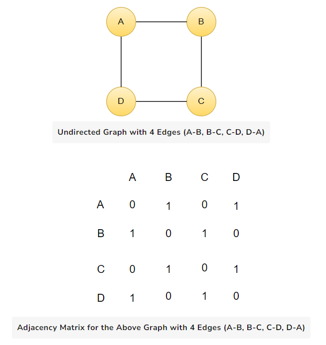
Adjacency matrix for undirected graphs

In an undirected graph with N vertices, the adjacency matrix A will be an N x N matrix. For an undirected edge between vertices i and j, the corresponding entries in the matrix (A[i][j] and A[j][i]) will have a value of 1, indicating the presence of an edge. If there is no edge between vertices i and j, the matrix entries will have the value of 0.

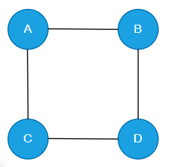
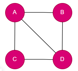
Example of an undirected graph with 4 vertices (A, B, C, D) and 4 edges (A-B, B-C, C-D, D-A):

Adjacency matrix for directed graphs

In a directed graph with N vertices, the adjacency matrix A will also be an N x N matrix. For a directed edge from vertex i to vertex j, the corresponding entry in the matrix () will have the value of 1, indicating the presence of an edge from i to j. If there is no edge from vertex i to vertex j, the matrix entry will have the value of 0.

Example of a directed graph with 4 vertices (A, B, C, D) and 5 directed edges (A->B, A->C, C->D, D->B, D->C):

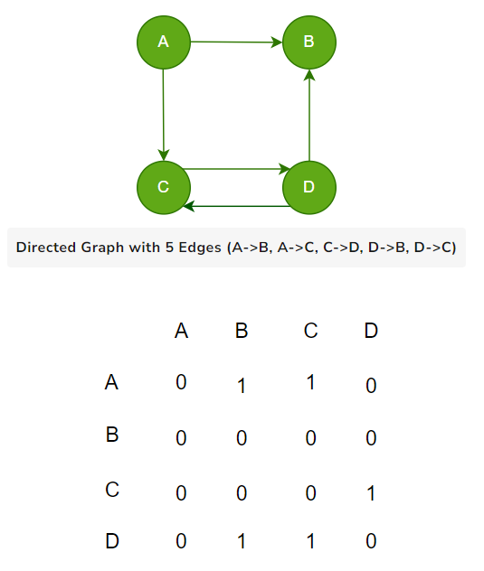
The above figure explains the adjacency matrix of the directed graph in such a way that there is an edge between vertices A-C and A-B so 1 is placed there.

Adjacency List

In linked list representation, an adjacency list is used to store the graph. An adjacency list is a common way to represent the connections between vertices in a graph. It is used in both directed and undirected graphs, but the way edges are stored and described differs slightly between the two types. In an adjacency list, each vertex is associated with a list of its neighboring vertices directly connected to it.

Representing undirected graph using adjacency list

In an undirected graph, the edges between vertices have no direction. If vertex A is connected to vertex B, then vertex B is also connected to vertex A. As a result, the adjacency list for an undirected graph is symmetric. Here is an example of a undirected graph with four vertices (A, B, C, D) and four edges.

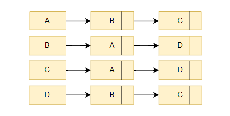
Here is the adjacency list for the above-undirected graph. From vertex A there is an edge to vertex B and C in the graph. So in the adjacency list, there are two nodes from node A.

Representing directed graphs using adjacency list

In a directed graph, the edges between vertices have a direction. If vertex X is connected to vertex Y, it does not necessarily mean that vertex Y is connected to vertex X. As a result, the adjacency list for a directed graph is not symmetric.

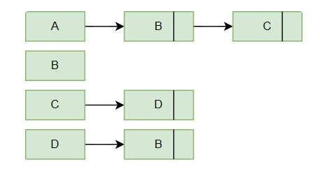
Example of a directed graph with 4 vertices (A, B, C, D) and 4 directed edges (A->B, A->C, C->D, D->B):

Here is the adjacency list for the above directed graph. From vertex A there is an edge to vertex B and C in the graph. So in the adjacency list, there are two nodes from node A. From vertex B there is no edge coming out so the adjacency list contains no further node from node B.

Graph as an Abstract Data Type (ADT)

As discussed earlier in the course, an abstract data type (ADT) is a theoretical concept that defines a set of operations and their behavior without specifying the internal representation of the data or the algorithms used to implement those operations. It provides a high-level description of the data and the functions that can be performed on it.

Here are some of the operations can be performed on graphs:

Adding a new vertex
Removing a vertex
Adding an edge between two vertices
Removing an edge between two vertices
Getting a list of all the vertices
Checking if two graph nodes are adjacent to each other or not
Getting count of the total vertices in the graph
Getting count of the total edges in the graph
Getting a list of the graph edges
Getting neighbors of a graph vertex

There are a few other ADT operations involving graph searching and traversal. Searching and traversal operations require detailed illustrations. Thereby, we will discuss those in the Graph Traversals section.

from collections import defaultdict

class Graph:
    def __init__(self):
        self.adjacencyList = {}

    def add_vertex(self, vertex):
        pass  # Add a new vertex to the graph.

    def remove_vertex(self, vertex):
        pass  # Remove a vertex from the graph.

    def add_edge(self, vertex1, vertex2):
        pass  # Add an edge between two vertices.

    def remove_edge(self, vertex1, vertex2):
        pass  # Remove an edge between two vertices.

    def get_vertices(self):
        return []  # Get a list of all vertices.

    def is_adjacent(self, vertex1, vertex2):
        return False  # Check if two vertices are adjacent.

    def get_vertex_count(self):
        return 0  # Get the total number of vertices.

    def get_edge_count(self):
        return 0  # Get the total number of edges.

    def get_edges(self):
        return []  # Get a list of all edges.

    def get_neighbors(self, vertex):
        return []  # Get a list of neighbors of a given vertex.

Implementing the ADT operations

In the beginning of this section, we mentioned ten major and the most common ADT operations associated with the graphs. Let’s discuss each operation individually - understanding how is it implemented.

1. add_vertex(vertex)

The function add_vertex(vertex) is a common operation in graph theory, where it adds a new vertex (also called a node or point) to a graph data structure. The vertex is a fundamental unit of a graph and represents an entity or an element. Adding a vertex expands the graph and creates potential connections (edges) between this new vertex and existing vertices.

In an adjacency list, each vertex is associated with a list of its adjacent vertices. We are using a dictionary or map for implementing the adjacency list. Thereby, we are able to store node key and value (s) associated with it.

For this course, we assume that graphs don’t have any extra satellite data or values associated with it. Therefore, we will add an empty vector or list as a value attribute for the new graph node or vertex.

You can add a new vertex following the two main steps:

Check if vertex already exists
- Use predefined map or dictionary search methods
If not, add it by inserting new key-value pair
- Keep value of the new inserted vertex as empty list

Here is a generalized pseudocode:

Graph is represented as:

adjacencyList (map/dictionary):
  key: vertex 
  value: list of adjacent vertices

Function addVertex(vertex)

  if vertex does not exist in adjacencyList
  
    add new key-value pair:
      key: vertex
      value: empty list     
    end if
    
end Function

Let’s now see the actual implementation of the add_vertex() method.

1
2
3

def add_vertex(self, vertex):
  if vertex not in self.adjacency_list:
    self.adjacency_list[vertex] = []

2. add_edge(vertex1, vertex2)

Pseudocode

Function addEdge(vertex1, vertex2):

  insert vertex2 into adjacencyList[vertex1]
  insert vertex1 into adjacencyList[vertex2]
  
end Function

To implement the add_edge() function, we need to add an edge between vertex1 and vertex2 in the graph. We are using the insert method provided by the std::unordered_map. This method allows us to insert elements into the vector of neighbors directly using an iterator.

Here is the implementation:

1
2
3

def add_edge(self, vertex1, vertex2):
     self.adjacency_list[vertex1].append(vertex2)
     self.adjacency_list[vertex2].append(vertex1)

A complete executable example

from collections import defaultdict

class Graph:
    def __init__(self):
        self.adjacency_list = defaultdict(list)

    def add_vertex(self, vertex):
        if vertex not in self.adjacency_list:
            self.adjacency_list[vertex] = []

    def remove_vertex(self, vertex):
        if vertex not in self.adjacency_list:
            return 
        self.adjacency_list.pop(vertex)
        for neighbors in self.adjacency_list.values():
            if vertex in neighbors:
                neighbors.remove(vertex)

    def add_edge(self, vertex1, vertex2):
        self.adjacency_list[vertex1].append(vertex2)
        self.adjacency_list[vertex2].append(vertex1)

    def remove_edge(self, vertex1, vertex2):
        self.adjacency_list[vertex1].remove(vertex2)
        self.adjacency_list[vertex2].remove(vertex1)
        
    def get_vertices(self):
        return list(self.adjacency_list.keys())
        
    def get_edges(self):
        edges = []
        for vertex, neighbors in self.adjacency_list.items():
            for neighbor in neighbors:

                if vertex < neighbor:
                    edges.append((vertex, neighbor))
        return edges
    
    def get_neighbors(self, vertex):
        return self.adjacency_list[vertex]

    def is_adjacent(self, vertex1, vertex2):
        return vertex2 in self.adjacency_list[vertex1]
    
    def get_vertex_count(self):
        return len(self.adjacency_list)
    
    def get_edge_count(self):
        count = sum(len(neighbors) for neighbors in self.adjacency_list.values())
        return count // 2
    
if __name__ == "__main__":
    graph = Graph()
    vertices = [1, 2, 3, 4, 5, 6]
    edges = [(1, 2), (1, 3), (2, 3), (3, 4), (4, 5), (5, 6)]

    for v in vertices:
        graph.add_vertex(v)

    for edge in edges:
        graph.add_edge(*edge)

    print(f"Vertices: {graph.get_vertices()}")
    print(f"Edges: {graph.get_edges()}")
    print(f"Neighbors of 1: {graph.get_neighbors(1)}")
    print(f"Is 1 adjacent to 2? {graph.is_adjacent(1, 2)}")

    graph.remove_edge(1, 2)
    graph.remove_vertex(3)

    print("After removing an edge and vertex:")
    print(f"Vertices: {graph.get_vertices()}") 
    print(f"Edges: {graph.get_edges()}")

Graph Traversal

A graph consists of vertices (nodes) connected by edges (lines). Graph traversal involves visiting all the graph nodes following a specific strategy or order. During traversal, each node is typically marked as visited to avoid revisiting the same node multiple times and to prevent infinite loops in cyclic graphs.

There are two common graph traversal algorithms: Depth-First Search (DFS) and Breadth-First Search (BFS). Let’s briefly discuss each of them:

Depth First Search(DFS)

Depth-First Search (DFS) is a graph traversal algorithm that explores all the nodes in a graph by systematically visiting as far as possible along each branch before backtracking. It operates on both directed and undirected graphs and can be implemented using recursion or an explicit stack data structure.

DFS starts from a selected source node (or a starting point) and explores as deeply as possible along each branch before backtracking. The algorithm visits nodes in a depth ward motion until it reaches a leaf node with no unexplored neighbors. At that point, it backtracks and explores other unexplored branches.

Here’s a step-by-step explanation of the DFS algorithm:

1. Initialization:

Choose a starting node as the source node.
Create a data structure to keep track of visited nodes (e.g., an array or a hash set) and mark the source node as visited.

2. Visit the Current Node:

Process the current node (e.g., print its value or perform any other operation you need to do).

3. Recursive Approach (Using Recursion):

For each unvisited neighbor of the current node:
- Recursively call the DFS function with the neighbor as the new current node.
- Mark the neighbor as visited.

4. Stack-Based Approach (Using an Explicit Stack):

Push the starting node onto the stack.
While the stack is not empty:
- Pop a node from the stack (current node).
- Process the current node (e.g., print its value or perform any other operation you need to do).
- For each unvisited neighbor of the current node:
  - Push the unvisited neighbor onto the stack.
  - Mark the neighbor as visited.

5. Backtracking:

If there are no more unvisited neighbors for the current node, backtrack by returning from the recursive function (if recursion) or popping nodes from the stack until a node with unvisited neighbors is found (if using an explicit stack).

6. Termination:

The DFS algorithm terminates when all nodes reachable from the source node have been visited. This means that all connected components of the graph have been explored.

Step-by-step Illustration of DFS

Let’s illustrate Depth-First Search (DFS) on a simple graph with its step-by-step traversal process.

Consider the following graph:

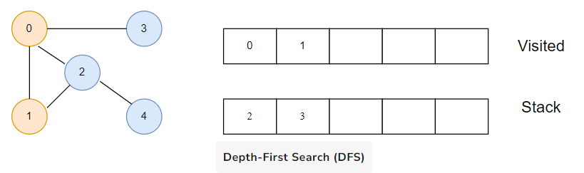
Depth-First Search (DFS) algorithm on an undirected graph with 5 vertices

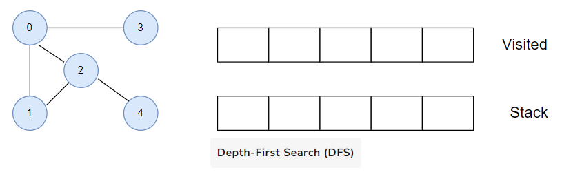
We are starting from vertex 0, the DFS algorithm starts by putting it in the visited list and putting all its adjacent vertices in the stack.

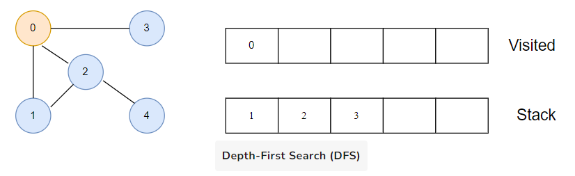
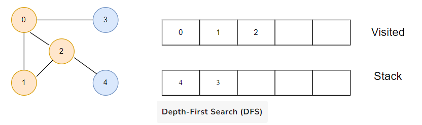
Next, we visit the element at the top of stack i.e. 1 and go to its adjacent nodes. Since 0 has already been visited, we visit 2 instead

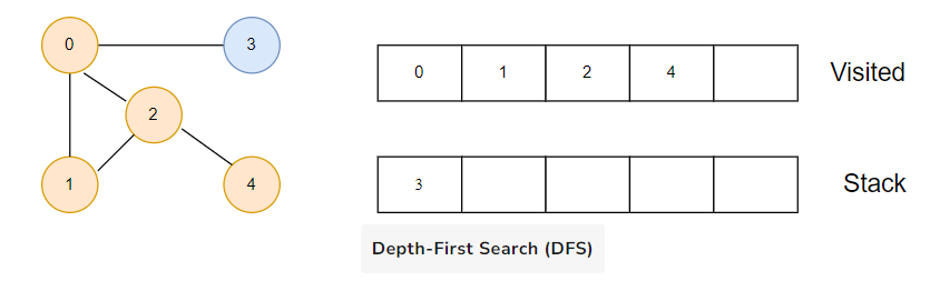
Vertex 2 has an unvisited adjacent vertex in 4, so we add that to the top of the stack and visit it.

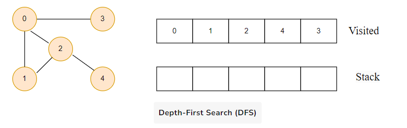
Next, we will visit 3.

After we visit the last element 3, it doesn’t have any unvisited adjacent nodes, so we have completed the Depth First Traversal of the graph.

Now, consider this example:

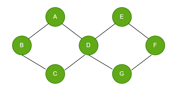
Starting from node A, let’s perform DFS on this graph:

Start at node A (the source node).
Mark node A as visited and process it: A (visited).
Explore an unvisited neighbor of A. Let’s say we choose B.
Mark node B as visited and process it: A -> B (visited).
From node B, explore an unvisited neighbor. We choose D.
Mark node D as visited and process it: A -> B -> D (visited).
Node D has no unvisited neighbors, so we backtrack to node B.
Node B has another unvisited neighbor, E. We explore E.
Mark node E as visited and process it: A -> B -> D -> E (visited).
From node E, explore an unvisited neighbor. We choose F.
Mark node F as visited and process it: A -> B -> D -> E -> F (visited).
Node F has no unvisited neighbors, so we backtrack to node E.
Node E has no more unvisited neighbors, so we backtrack to node B.
Node B has no more unvisited neighbors, so we backtrack to node A.
Node A has one more unvisited neighbor, C. We explore C.
Mark node C as visited and process it: A -> B -> D -> E -> F -> C (visited).
Node C has no unvisited neighbors, so we backtrack to node A.
Node A has no more unvisited neighbors, and we have visited all reachable nodes.

The DFS traversal order for this graph starting from node A is: A -> B -> D -> E -> F -> C.

Note that the choice of the starting node can affect the order of traversal for the graph. Also, in a disconnected graph, you would need to start DFS from each unvisited node to traverse all components.

Implementation of Depth First Search

Below is an implementation of Depth-First Search (DFS) in C++, Python, Java, and JavaScript. DFS is a graph traversal algorithm that explores as far as possible along each branch before backtracking.

In this example implementation, we assume that the graph is represented as an adjacency list.

class Graph:
    def __init__(self, V):
        self.vertices = V
        self.adjList = [[] for _ in range(V)]

    def addEdge(self, u, v):
        self.adjList[u].append(v)
        self.adjList[v].append(u)  # For an undirected graph

    def DFS(self, start):
        visited = [False] * self.vertices
        stack = []

        stack.append(start)
        visited[start] = True

        while stack:
            curr = stack.pop()
            print(curr)

            for neighbor in self.adjList[curr]:
                if not visited[neighbor]:
                    stack.append(neighbor)
                    visited[neighbor] = True

g = Graph(7)

g.addEdge(0, 1)
g.addEdge(0, 2)
g.addEdge(1, 3)
g.addEdge(1, 4)
g.addEdge(2, 5)
g.addEdge(2, 6)

print("DFS Traversal starting from vertex 0:")
g.DFS(0)

Complexity analysis

The time and space complexity of Depth-First Search (DFS) depend on the size and structure of the graph being traversed. Let’s analyze the complexity of DFS:

1. Time Complexity:

In the worst case, DFS once visits all nodes and edges in the graph. For a graph with V vertices (nodes) and E edges, the time complexity of DFS is O(V + E)
The time complexity can be further broken down as follows:
- Visiting a node (marking it as visited and processing it) takes O(1) time.
- Exploring all neighbors of a node takes O(d) time, where ‘d’ is the average degree of nodes in the graph. In the worst case, ‘d’ can be as high as V - 1 (complete graph).
  - So, the time complexity can be approximated as O(V) for exploring all neighbors of one node.

In summary, the overall time complexity of DFS is: O(V + E)

2. Space Complexity:

The space complexity of DFS is determined by the space needed to store information about the nodes during the traversal. The primary sources of space usage are the recursion stack (if using recursion) or the explicit stack data structure (if using an iterative approach).
In the worst case, the maximum depth of the recursion stack (or the maximum number of nodes stored in the stack) is the height of the deepest branch of the graph. For a graph with a single connected component, this height can be O(V - 1) (when all nodes are connected in a straight line).
The space complexity of the recursion stack in the worst case is O(V). Additionally, if an explicit stack is used, its space complexity would also be O(V) in the worst case.

In summary, the overall space complexity of DFS is O(V) due to the recursion stack or the explicit stack.

DFS can be used for various applications, such as finding connected components, detecting cycles in the graph, topological sorting, and solving problems like maze exploration or finding paths between nodes.

It’s essential to be cautious about infinite loops when traversing graphs that may have cycles. To avoid this, the algorithm must keep track of visited nodes and avoid revisiting nodes that have already been explored.

Overall, DFS is a powerful graph traversal algorithm that can efficiently explore the entire graph and is widely used in many graph-related problems.

Breadth First Search (BFS)

Breadth-First Search (BFS) is a graph traversal algorithm that explores a graph’s vertices (nodes) level by level. It starts from a selected source node and moves outward to visit all the nodes at the same distance from the source before moving on to nodes at the following distance level.

BFS is particularly useful for finding the shortest path in unweighted graphs and for systematically exploring graphs.

Here is a complete description of the Breadth-First Search algorithm:

1. Use a Queue

BFS uses a queue to keep track of the nodes to be visited. The queue follows the First-In-First-Out (FIFO) principle, where the first node inserted in the queue will be the first one to be removed (dequeue).

2. Initialization:

Start by selecting a source node to begin the traversal.
Create an empty queue to hold the nodes to be visited.
Mark the source node as visited and enqueue it into the queue.

3. Traversal:

While the queue is not empty, continue the following steps:
- Dequeue a node from the front of the queue (let’s call it the “current node”).
- Process the current node (print it, perform some operation, etc.).
- Enqueue all the unvisited neighbors of the current node into the queue.
- Mark each enqueued neighbor as visited.

4. Termination:

The BFS algorithm continues until the queue becomes empty, meaning all reachable nodes from the source node have been visited.

Step-by-Step Illustration of BFS

Let’s see how the Breadth First Search algorithm works with an example. We use an undirected graph with 5 vertices.

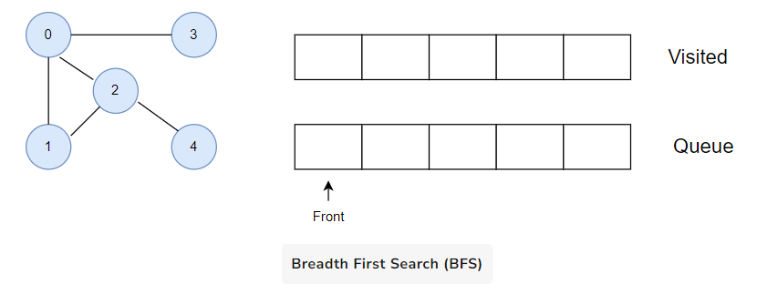
We start from vertex 0, the BFS algorithm starts by putting it in the Visited list and putting all its adjacent vertices in the queue.

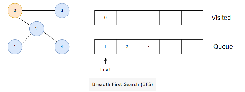
Next, we visit the element at the front of queue i.e. 1 and go to its adjacent nodes. Since 0 has already been visited, we visit 2 instead.

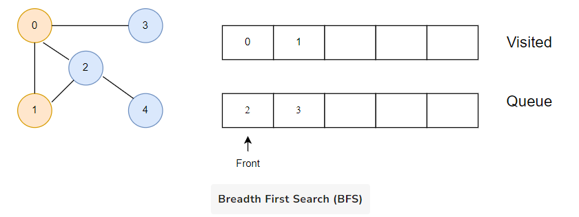
Vertex 2 has an unvisited adjacent vertex in 4, so we add that to the back of the queue and visit 3, which is at the front of the queue.

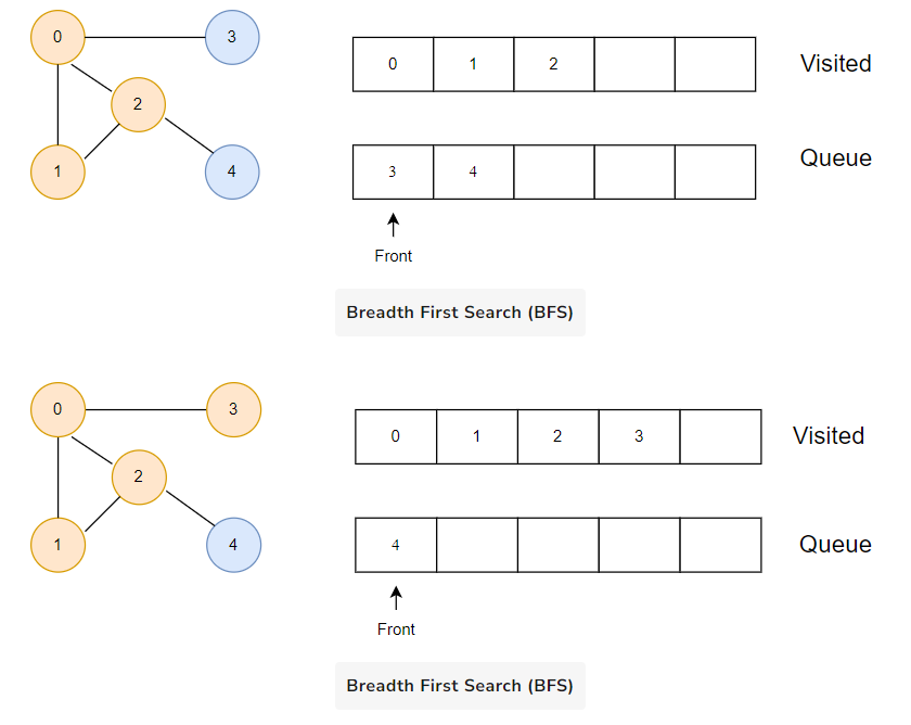
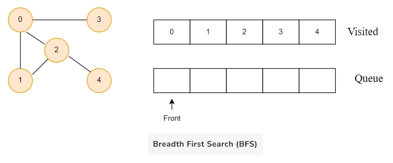
Only 4 remains in the queue since the only adjacent node of 3 i.e. 0 is already visited. We visit it.

Now, consider this example:

Starting from the source node A, the BFS traversal would be as follows:

Start with A (the source node) and enqueue it. Queue: [A]
Dequeue A and process it. Enqueue its neighbors B and C. Queue: [B, C]
Dequeue B and process it. Enqueue its neighbors D and E. Queue: [C, D, E]
Dequeue C and process it. Enqueue its neighbor F. Queue: [D, E, F]
Dequeue D and process it. No unvisited neighbors to enqueue. Queue: [E, F]
Dequeue E and process it. Enqueue its neighbor F. Queue: [F]
Dequeue F and process it. No unvisited neighbors to enqueue. Queue: []

The BFS traversal order is: A -> B -> C -> D -> E -> F.

BFS guarantees that it visits nodes in the order of their distance from the source node.

It is an efficient algorithm to find the shortest path in unweighted graphs. Additionally, BFS can be used to find connected components, detect cycles, and solve various graph-related problems. However, it may consume more memory compared to DFS, especially in graphs with a large branching factor or infinite graphs.

Implementation of Breadth First Search

Below is an implementation of Breadth-First Search (DFS) in C++, Python, Java, and JavaScript. BFS is an algorithm used for traversing or searching a graph or tree in a level-by-level manner.

from collections import defaultdict, deque

class Graph:
    def __init__(self, vertices):
        self.V = vertices
        self.adjList = defaultdict(list)

    def addEdge(self, u, v):
        self.adjList[u].append(v)
        self.adjList[v].append(u)  # For undirected graph

    def BFS(self, startVertex):
        visited = [False] * self.V  # To keep track of visited vertices
        q = deque()

        visited[startVertex] = True
        q.append(startVertex)

        while q:
            currentVertex = q.popleft()
            print(currentVertex, end=" ")

            # Explore adjacent vertices
            for neighbor in self.adjList[currentVertex]:
                if not visited[neighbor]:
                    visited[neighbor] = True
                    q.append(neighbor)

if __name__ == "__main__":
    graph = Graph(6)  # Create a graph with 6 vertices

    graph.addEdge(0, 1)
    graph.addEdge(0, 2)
    graph.addEdge(1, 3)
    graph.addEdge(2, 4)
    graph.addEdge(3, 4)
    graph.addEdge(3, 5)

    print("Breadth-First Traversal starting from vertex 0:")
    graph.BFS(0)

Complexity analysis

The time and space complexity of Breadth-First Search (BFS) depends on the size of the graph and the way it is represented. Let’s analyze the complexities:

1. Time Complexity:

Visiting a vertex takes O(1) time as we dequeue it from the queue in constant time.
Exploring the neighbors of a vertex takes O(1) time per neighbor, as we have to traverse its adjacency list once.
In the worst case, we visit all the vertices at least once, which takes O(V) time. Additionally, for each vertex, we explore all its neighbors once, which takes O(E) time in total (sum of the sizes of all adjacency lists).
Hence, the overall time complexity of BFS is: O(V + E)

2. Space Complexity:

The space required to store the graph using an adjacency list representation is O(V + E), as we need to store each vertex and its corresponding edges.
The space required for the queue in BFS is O(V) in the worst case, as all the vertices can be in the queue at once.
Since the space occupied by the queue is dominant in the overall space complexity, the space complexity of BFS is: O(V)

BFS is generally efficient for searching and traversal when the graph is not too dense. For sparse graphs, where E is much smaller than V^2, the time complexity becomes almost linear, making BFS a reasonable choice for many practical applications.

BFS guarantees it visits nodes according to their distance from the source node. It is an efficient algorithm to find the shortest path in unweighted graphs. Additionally, BFS can find connected components, detect cycles, and solve graph-related problems. However, it may consume more memory than DFS, especially in graphs with a significant or infinite branching factor.

Find if Path Exists in Graph(easy)

1971. Find if Path Exists in Graph Design Gurus

Problem Statement

Given an undirected graph, represented as a list of edges. Each edge is illustrated as a pair of integers [u, v], signifying that there’s a mutual connection between node u and node v.

Given this graph, a starting node start, and a destination node end, your task is to ascertain if a path exists between the starting node and the destination node.

Examples

Example 1:
- Input: 4, [[0,1],[1,2],[2,3]], 0, 3
- Expected Output: true
- Justification: There’s a path from node 0 -> 1 -> 2 -> 3.
Example 2:
- Input: 4, [[0,1],[2,3]], 0, 3
- Expected Output: false
- Justification: Nodes 0 and 3 are not connected, so no path exists between them.
Example 3:
- Input: 5, [[0,1],[3,4]], 0, 4
- Expected Output: false
- Justification: Nodes 0 and 4 are not connected in any manner.

Constraints:

1 <= n <= 2 * 10^5
0 <= edges.length <= 2 * 10^5
edges[i].length == 2
0 <= ui, vi <= n - 1
ui != vi
0 <= source, destination <= n - 1
There are no duplicate edges.
There are no self edges.

Solution

The task at hand is to determine if there’s a path from a starting node to an ending node in a given undirected graph. Our approach uses Depth First Search (DFS) to explore the graph recursively. Starting at the initial node, we’ll dive as deep as possible into its neighboring nodes. If we reach the target node at any point during the traversal, we know a path exists. If we exhaust all possible routes and haven’t found the target, then no path exists.

Graph Representation: We’ll begin by converting the provided edge list into an adjacency list to represent our graph. The adjacency list is essentially an array (or list) of lists, where each index corresponds to a node, and its content is a list of neighbors for that node. Since our graph is undirected, if there’s an edge between nodes A and B, both A will be in B’s list and B in A’s list.
Depth First Search (DFS): With our graph ready, we then use a recursive DFS function to traverse the graph. This function starts at the given node, and if it’s the target node, we return true. Otherwise, we mark this node as visited and call the DFS function on all its unvisited neighbors. This dives deeper into the graph. If any of these recursive calls return true (meaning they found the target), our current DFS call also returns true.
Handling Cycles: To avoid getting stuck in a loop, especially in cyclic graphs, we keep track of which nodes we’ve visited. Before exploring a node, we’ll check if it’s been visited; if it has, we’ll skip it.
Result: If our DFS exploration reaches the target node, we return true, signifying that a path exists. Otherwise, after checking all paths from the starting node and not finding the target, we’ll conclude and return false.

Algorithm Walkthrough: Using the input from Example 1:

Nodes = 4, Edges = [[0,1],[1,2],[2,3]], Start = 0, End = 3

Create the graph from the edges.
Begin DFS at node 0.
Mark node 0 as visited.
Explore neighbors of node 0. Discover node 1.
Delve into DFS for node 1.
Mark node 1 as visited.
Explore neighbors of node 1. Discover node 2.
Delve into DFS for node 2.
Mark node 2 as visited.
Explore neighbors of node 2. Discover node 3.
Since node 3 is the target end node, return true.

Code

Here is the code for this algorithm:

# 官方使用递归如下，但是我更习惯我写的，使用while
from collections import defaultdict

class Solution:
    def validPath(self, n: int, edges: [[int]], start: int, end: int) -> bool:
        graph = defaultdict(list)
        
        # Create graph from edges
        for u, v in edges:
            graph[u].append(v)
            graph[v].append(u)  # Undirected graph
        
        visited = set()

        def dfs(node):
            if node == end:  # Found the path
                return True
            visited.add(node)
            
            # Traverse neighbors
            for neighbor in graph[node]:
                if neighbor not in visited and dfs(neighbor):
                    return True
            return False  # Path not found

        return dfs(start)

# Test
sol = Solution()
print(sol.validPath(4, [[0,1],[1,2],[2,3]], 0, 3))  # true
print(sol.validPath(4, [[0,1],[2,3]], 0, 3))      # false
print(sol.validPath(5, [[0,1],[3,4]], 0, 4))      # false


# 自己写的，可以过leetcode
from collections import defaultdict, deque


class Solution:
    def validPath(self, n: int, edges: [[int]], start: int, end: int) -> bool:
        graph = {i: [] for i in range(n)}

        # Create graph from edges
        for u, v in edges:
            graph[u].append(v)
            graph[v].append(u)  # Undirected graph

        visited = [False for i in range(n)]
        stack = deque()
        stack.append(start)
        visited[start] = True
        while stack:
            element = stack.pop()
            for child in graph[element]:
                if not visited[child]:
                    stack.append(child)
                    visited[child] = True
                if child == end:
                    return True
        return False


# Test
sol = Solution()
print(sol.validPath(4, [[0, 1], [1, 2], [2, 3]], 0, 3))  # true
print(sol.validPath(4, [[0, 1], [2, 3]], 0, 3))  # false
print(sol.validPath(5, [[0, 1], [3, 4]], 0, 4))  # false

Time Complexity

Graph Construction: Constructing the adjacency list from the given edge list takes (O(E)), where (E) is the number of edges. Each edge is processed once.
DFS Traversal: In the worst-case scenario, the Depth-First Search (DFS) can traverse all nodes and all edges once. This traversal has a time complexity of (O(V + E)), where (V) is the number of vertices or nodes, and (E) is the number of edges.

Combining the above, our time complexity is dominated by the DFS traversal, making it (O(V + E)).

Space Complexity

Graph Representation: The adjacency list requires (O(V + E)) space.
Visited Set/Array: The visited set (or array) will take (O(V)) space, as it needs to track each node in the graph.
Recursive Call Stack: The DFS function is recursive, and in the worst case (for a connected graph), it can have (V) nested calls. This would result in a call stack depth of (V), adding (O(V)) space complexity.

The dominant factor here is the graph representation and the call stack, so the total space complexity is (O(V + E)).

Summary:

Time Complexity: (O(V + E))
Space Complexity: (O(V + E))

This makes our algorithm efficient, especially for sparse graphs (i.e., graphs with relatively fewer edges compared to nodes). The worst-case scenario is when the graph is fully connected, but even then, our algorithm is designed to handle it within reasonable limits.

Number of Provinces (medium)

547. Number of Provinces Design Gurus

也可以使用并查集，在Pattern Union Find中

Problem Statement

Imagine a country with several cities. Some cities have direct roads connecting them, while others might be connected through a sequence of intermediary cities. Using a matrix representation, if matrix[i][j] holds the value 1, it indicates that city i is directly linked to city j and vice versa. If it holds 0, then there’s no direct link between them.

Determine the number of separate city clusters (or provinces).

A province is defined as a collection of cities that can be reached from each other either directly or through other cities in the same province.

Examples

- Input:
  1
  [[1,1,0],[1,1,0],[0,0,1]]
- Expected Output:
  2
- Justification:
  There are two provinces: cities 0 and 1 form one province, and city 2 forms its own province.
- Input:
  1
  [[1,0,0,1],[0,1,1,0],[0,1,1,0],[1,0,0,1]]
- Expected Output:
  2
- Justification:
  There are two provinces: cities 0 and 3 are interconnected forming one province, and cities 1 and 2 form another.
- Input:
  1
  [[1,0,0],[0,1,0],[0,0,1]]
- Expected Output:
  3
- Justification:
  Each city stands alone and is not connected to any other city. Thus, we have three provinces.

Constraints:

1 <= n <= 200
n == isConnected.length
n == isConnected[i].length
isConnected[i][j] is 1 or 0.
isConnected[i][i] == 1
isConnected[i][j] == isConnected[j][i]

Solution

At a high level, the problem of identifying provinces in the given matrix can be visualized as detecting connected components in an undirected graph. Every city represents a node, and a direct connection between two cities is an edge. The number of separate, interconnected clusters in this graph is essentially the number of provinces. To navigate this graph and identify these clusters, we employ the Depth First Search (DFS) technique, marking visited nodes (cities) along the way.

Initialization: Start with a visited array, initialized with all values set to false. This will help in keeping track of cities that have been processed.
DFS Function: This recursive function allows us to traverse the matrix. When an unvisited city is found, we recursively visit all other cities accessible from it, marking them as visited. All cities traversed in a single DFS invocation belong to the same province.
Counting Provinces: Every unique invocation of the DFS function on an unvisited city, from the main function, signifies the discovery of a new province. Therefore, for each such invocation, we increment our province count.
Completion: After every city has been visited, our province counter will hold the total number of provinces in the country.

Algorithm Walkthrough: Using the input [[1,1,0],[1,1,0],[0,0,1]]:

Begin with an unvisited visited array: [false, false, false].
Start from city 0:
- Visit city 0 and city 1 since they are connected. Update visited to [true, true, false].
City 2 remains unvisited, but it isn’t connected to any other unvisited city. So, it forms its own province.
We initiated the DFS twice: once for the province comprising cities {0,1} and once for the solitary city 2.
Our answer becomes 2.

Code

Here is the code for this algorithm:

# 官方使用的是递归
class Solution:
    def findCircleNum(self, isConnected) -> int:
        def dfs(city):
            # For each city, mark it as visited and explore its connections
            for i in range(len(isConnected)):
                if isConnected[city][i] == 1 and not visited[i]:
                    visited[i] = True
                    dfs(i)

        visited = [False] * len(isConnected)
        provinces = 0

        for city in range(len(isConnected)):
            if not visited[city]:
                dfs(city)
                provinces += 1

        return provinces

# Test the Solution class
solution = Solution()
print(solution.findCircleNum([[1,1,0], [1,1,0], [0,0,1]]))  # Expected output: 2
print(solution.findCircleNum([[1,0,0,1], [0,1,1,0], [0,1,1,0], [1,0,0,1]]))  # Expected output: 2
print(solution.findCircleNum([[1,0,0], [0,1,0], [0,0,1]]))  # Expected output: 3

Time Complexity

Depth First Search (DFS): For a given node, the DFS will explore all of its neighbors. In the worst case, we may end up visiting all nodes in the graph starting from a single node. Hence, the DFS complexity is (O(n)), where (n) is the number of nodes.
Overall Time Complexity: For each node, we might call DFS once (if that node is not visited before). Thus, the overall time complexity is (O(n^2)), with the DFS call being nested inside a loop that iterates over all nodes. In dense graphs where each node is connected to every other node, we will reach this upper bound.

Space Complexity

Visited Array: This is an array of size (n) (the number of nodes), so its space requirement is (O(n)).
Recursive Call Stack: In the worst case, if all cities are connected in a linear manner (like a linked list), the maximum depth of recursive DFS calls will be (n). Hence, the call stack will take (O(n)) space.
Overall Space Complexity: The dominant space-consuming factors are the visited array and the recursive call stack. Hence, the space complexity is (O(n)).

In summary:

Time Complexity: (O(n^2))
Space Complexity: (O(n))

This algorithm is efficient because once a city is visited, it won’t be visited again, ensuring we don’t do redundant work. Moreover, using DFS allows us to deeply traverse through connected cities, marking entire provinces in one go. This approach optimizes our search and helps in reducing the number of unnecessary computations.

Minimum Number of Vertices to Reach All Nodes(medium)

1557. Minimum Number of Vertices to Reach All Nodes Design Gurus 这道题适合在拓扑排序中

Problem Statement

Given a directed acyclic graph with n nodes labeled from 0 to n-1, determine the smallest number of initial nodes such that you can access all the nodes by traversing edges. Return these nodes.

Examples

Input:
- n = 6
- edges = [[0,1],[0,2],[2,5],[3,4],[4,2]]
Expected Output: [0,3]

Justification: Starting from nodes 0 and 3, you can reach all other nodes in the graph. Starting from node 0, you can reach nodes 1, 2, and 5. Starting from node 3, you can reach nodes 4 and 2 (and by extension 5).
Input:
- n = 3
- edges = [[0,1],[2,1]]
Expected Output: [0,2]

Justification: Nodes 0 and 2 are the only nodes that don’t have incoming edges. Hence, you need to start from these nodes to reach node 1.
Input:
- n = 5
- edges = [[0,1],[2,1],[3,4]]
Expected Output: [0,2,3]

Justification: Node 1 can be reached from both nodes 0 and 2, but to cover all nodes, you also need to start from node 3.

Constraints:

2 <= n <= 10^5
1 <= edges.length <= min(10^5, n * (n - 1) / 2)
edges[i].length == 2
0 <= fromi, toi < n
All pairs (fromi, toi) are distinct.

Solution

To solve the problem of determining the minimum number of vertices needed to reach all nodes in a directed graph, we focus on the concept of “in-degree” which represents the number of incoming edges to a node. In a directed graph, if a node doesn’t have any incoming edges (in-degree of 0), then it means that the node cannot be reached from any other node. Hence, such nodes are mandatory starting points to ensure that every node in the graph can be reached. Our algorithm thus identifies all nodes with an in-degree of 0 as they are potential starting points to traverse the entire graph.

Steps:

Graph Representation: Begin by representing the graph using an adjacency list or a similar data structure.
In-Degree Calculation: Compute the in-degree for all the nodes. The in-degree of a node is the number of edges coming into it. This can be done by initializing an array to keep track of in-degrees for each node and iterating over the edges to update the in-degree counts.
Result Gathering: Iterate over the computed in-degrees. Nodes with an in-degree of 0 don’t have any incoming edges and thus are part of our result set as they serve as starting points.

Algorithm Walkthrough:

Let’s walk through the solution using the example n = 6 and edges = [[0,1],[0,2],[2,5],[3,4],[4,2]]:

Step 1: Start with an in-degree array initialized to zeros for all nodes: [0, 0, 0, 0, 0, 0].
Step 2: Iterate over the edges. For each edge (source, destination), increment the in-degree of the destination node by 1. After processing all edges, the in-degree array becomes: [0,1,2,0,1,1].
Step 3: Finally, by examining the in-degree array, nodes 0 and 3 are identified as having an in-degree of 0. This means they don’t receive any incoming edges, and thus, they become our result set: [0,3]. Starting from these nodes, we can reach all other nodes in the graph.

Code

Here is the code for this algorithm:

from typing import List

class Solution:
    def findSmallestSetOfVertices(self, n: int, edges: List[List[int]]) -> List[int]:
        # Create a set to store nodes with incoming edges
        nodes_with_incoming = set()
        
        # Populate the set
        for _, to_node in edges:
            nodes_with_incoming.add(to_node)
        
        # Return nodes without incoming edges
        return [i for i in range(n) if i not in nodes_with_incoming]

if __name__ == "__main__":
    solution = Solution()
    
    # Test cases
    edges1 = [[0,1], [0,2], [2,5], [3,4], [4,2]]
    print(solution.findSmallestSetOfVertices(6, edges1))  # Expected: [0, 3]
    
    edges2 = [[0,1], [3,1], [1,2]]
    print(solution.findSmallestSetOfVertices(4, edges2))  # Expected: [0, 3]
    
    edges3 = [[2,0], [3,2]]
    print(solution.findSmallestSetOfVertices(4, edges3))  # Expected: [1, 3]

Time Complexity:

Initialization: Initializing the set for all nodes in the graph takes (O(n)), where (n) is the number of nodes.
Processing Edges: For every edge ([u, v]), we are simply checking and potentially removing the node (v) from our set. Since we do a constant amount of work for each edge, this step takes (O(e)) time, where (e) is the number of edges.

Thus, the overall time complexity is the sum of the above two steps, i.e., (O(n + e)). In the worst case (a complete graph), every node is connected to every other node, making (e = n^2), leading to a worst-case time complexity of (O(n^2)). However, this is not a typical scenario, and in most real-world graphs, (e) is often linear or close to linear with respect to (n). Therefore, (O(n + e)) is a more informative measure.

Space Complexity:

Set for Nodes: The set that we’re using to keep track of nodes which do not have any incoming edges will, at most, contain all nodes. This gives us a space complexity of (O(n)).
Graph Representation: Though we are given the edges as an input, if we consider the space used by this representation, it will be (O(e)) for the edges.

However, note that since we are not using any additional data structures that scale with the size of the graph other than the set for nodes, our primary concern is the set’s space. Thus, the dominant term here is (O(n)).

So, the overall space complexity is (O(n)).

In summary: