
Daily Temperatures
Problem Statement
You are given a list of daily temperatures. Your task is to return an answer array such that answer[i] is the number of days you would have to wait until a warmer temperature for each of the days. If there is no future day for which this is possible, put 0 instead.
Examples
- Input: [45, 50, 40, 60, 55]
- Expected Output: [1, 2, 1, 0, 0]
- Justification: The next day after the first day is warmer (50 > 45). Two days after the second day, the temperature is warmer (60 > 50).. The next day after the third day is warmer (60 > 40). There are no warmer days after the fourth and fifth days.
- Input: [80, 75, 85, 90, 60]
- Expected Output: [2, 1, 1, 0, 0]
- Justification: Two days after the first day, the temperature is warmer (85 > 80). The next day after the second day is warmer (85 > 75). The next day after the third day is warmer (90 > 85). There are no warmer days after the fourth and fifth days.
- Input: [32, 32, 32, 32, 32]
- Expected Output: [0, 0, 0, 0, 0]
- Justification: All the temperatures are the same, so there are no warmer days ahead.
Constraints:
- 1 <= temperatures.length <= 105
30 <= temperatures[i] <= 100
Solution
- Understanding the Problem:
- The problem is to find the number of days until a warmer day for each day in the list.
- Approach:
- Use a stack to keep track of the indices of the days.
- Iterate through the list of temperatures.
- While the stack is not empty and the current temperature is greater than the temperature at the index at the top of the stack:
- Pop an index from the stack and calculate the difference between the current day and the popped index.
- Store this difference at the popped index in the result array.
- Push the current day’s index onto the stack.
- While the stack is not empty and the current temperature is greater than the temperature at the index at the top of the stack:
- Why This Works:
- The stack keeps track of the days for which a warmer day has not yet been found.
- When a warmer day is found, the days are popped from the stack and the difference in days is calculated.
Algorithm Walkthrough
Consider the input [45, 50, 40, 60, 55]:
- Initialize an empty stack and a result array filled with zeros:
stack = [], res = [0, 0, 0, 0, 0]. - Iterate through the list:
- Day 1 (45):
stack = [0]. - Day 2 (50): Pop
0fromstack,res[0] = 1 - 0 = 1,stack = [1]. - Day 3 (40):
stack = [1, 2]. - Day 4 (60): Pop
2fromstack,res[2] = 3 - 2 = 1, Pop1fromstack,res[1] = 3 - 1 = 2,stack = [3]. - Day 5 (55):
stack = [3, 4].
- Day 1 (45):
- End of iteration,
res = [1, 2, 1, 0, 0].
Code Development
1 | class Solution: |
Complexity Analysis
- Time Complexity: O(n), where n is the number of temperatures. This is because the algorithm iterates through the list of temperatures once, performing constant-time operations for each temperature.
- Space Complexity: O(n), as it uses a stack to keep track of indices.
Group Anagrams
Problem Statement
Given a list of strings, the task is to group the anagrams together.
An anagram is a word or phrase formed by rearranging the letters of another, such as “cinema”, formed from “iceman”.
Example Generation
Example 1:
- Input:
["dog", "god", "hello"] - Output:
[["dog", "god"], ["hello"]] - Justification: “dog” and “god” are anagrams, so they are grouped together. “hello” does not have any anagrams in the list, so it is in its own group.
Example 2:
- Input:
["listen", "silent", "enlist"] - Output:
[["listen", "silent", "enlist"]] - Justification: All three words are anagrams of each other, so they are grouped together.
Example 3:
- Input:
["abc", "cab", "bca", "xyz", "zxy"] - Output:
[["abc", "cab", "bca"], ["xyz", "zxy"]] - Justification: “abc”, “cab”, and “bca” are anagrams, as are “xyz” and “zxy”.
Constraints:
- 1 <= strs.length <= 10^4
0 <= strs[i].length <= 100strs[i]consists of lowercase English letters.
Solution
- Sorting Approach:
- For each word in the input list:
- Sort the letters of the word.
- Use the sorted word as a key in a hash map, and add the original word to the list of values for that key.
- The hash map values will be the groups of anagrams.
- For each word in the input list:
- Why This Will Work:
- Anagrams will always result in the same sorted word, so they will be grouped together in the hash map.
Algorithm Walkthrough
- Given the input
["abc", "cab", "bca", "xyz", "zxy"] - For “abc”:
- Sorted word is “abc”.
- Add “abc” to the hash map with key “abc”.
- For “cab”:
- Sorted word is “abc”.
- Add “cab” to the list in the hash map with key “abc”.
- Continue this process for all words.
- The hash map values are the groups of anagrams.
Code
1 | class Solution: |
Complexity Analysis
- Time Complexity: O(nklog(k)), where n is the number of strings, and k is the maximum length of a string in strs. This is because each of the n strings is sorted in O(k*log(k)) time.
- Space Complexity: O(n*k), where n is the number of strings, and k is the maximum length of a string in strs. This space is used for the output data structure and the hash map.
Decode String
Problem Statement
You have a string that represents encodings of substrings, where each encoding is of the form k[encoded_string], where k is a positive integer, and encoded_string is a string that contains letters only.
Your task is to decode this string by repeating the encoded_string k times and return it. It is given that k is always a positive integer.
Examples
- Input:
"3[a3[c]]" - Expected Output:
"acccacccaccc" - Justification: The inner
3[c]is decoded asccc, and thenais appended to the front, formingacc. This is then repeated 3 times to formacccacccaccc.
- Input:
- Input:
"2[b3[d]]" - Expected Output:
"bdddbddd" - Justification: The inner
3[d]is decoded asddd, and thenbis appended to the front, formingbddd. This is then repeated 2 times to formbddd bddd.
- Input:
- Input:
"4[z]" - Expected Output:
"zzzz" - Justification: The
4[z]is decoded aszrepeated 4 times, formingzzzz.
- Input:
Constraints:
1 <= s.length <= 30sconsists of lowercase English letters, digits, and square brackets ‘[]’.sis guaranteed to be a valid input.- All the integers in s are in the range
[1, 300].
Solution
- Understanding the Problem:
- The problem involves decoding a string that contains patterns where a number is followed by a string in brackets.
- The number indicates how many times the string in brackets should be repeated.
- Approach:
- Use a stack to keep track of the characters in the string.
- Iterate through the string character by character.
- When a number is encountered, calculate the complete number.
- When an opening bracket
[is encountered, push the calculated number to the stack. - When a closing bracket
]is encountered, pop elements from the stack until a number is encountered and form the substring to be repeated. - Multiply the substring with the number and push the result back to the stack.
- Handling Nested Brackets:
- The stack will naturally handle nested brackets as it will continue popping elements until a number is encountered, forming the substring for the innermost bracket first.
Algorithm Walkthrough
- Given Input:
"3[a3[c]]" - Steps:
- Initialize an empty stack.
- Iterate through the string:
- Encounter
3, push3to the stack. - Encounter
[, do nothing. - Encounter
a, pushato the stack. - Encounter
3, push3to the stack. - Encounter
[, do nothing. - Encounter
c, pushcto the stack. - Encounter
], popcand3, formcccand push it back to the stack. - Encounter
], popccc,a, and3, formacccacccacccand push it back to the stack.
- Encounter
- The final stack contains
acccacccacccas the only element, which is the decoded string.
Code
1 | class Solution: |
Complexity Analysis
- Time Complexity: O(n), where n is the length of the input string. This is because we are iterating through the string once and processing each character.
- Space Complexity: O(n), where n is the length of the input string. In the worst case, the stack will store all the characters of the input string.
Valid Sudoku
Problem Statement
Determine if a 9x9 Sudoku board is valid. A valid Sudoku board will hold the following conditions:
- Each row must contain the digits 1-9 without repetition.
- Each column must contain the digits 1-9 without repetition.
- The 9 3x3 sub-boxes of the grid must also contain the digits 1-9 without repetition.
Note:
- The Sudoku board could be partially filled, where empty cells are filled with the character ‘.’.
- You need to validate only filled cells.
Example 1:
Input:
1
2
3
4
5
6
7
8
9[["5","3",".",".","7",".",".",".","."]
,["6",".",".","1","9","5",".",".","."]
,[".","9","8",".",".",".",".","6","."]
,["8",".",".",".","6",".",".",".","3"]
,["4",".",".","8",".","3",".",".","1"]
,["7",".",".",".","2",".",".",".","6"]
,[".","6",".",".",".",".","2","8","."]
,[".",".",".","4","1","9",".",".","5"]
,[".",".",".",".","8",".",".","7","9"]]Expected Output:
trueJustification: This Sudoku board is valid as it adheres to the rules of no repetition in each row, each column, and each 3x3 sub-box.
Example 2:
Input:
1
2
3
4
5
6
7
8
9[["8","3",".",".","7",".",".",".","."]
,["6",".",".","1","9","5",".",".","."]
,[".","9","8",".",".",".",".","6","."]
,["8",".",".",".","6",".",".",".","3"]
,["4",".",".","8",".","3",".",".","1"]
,["7",".",".",".","2",".",".",".","6"]
,[".","6",".",".",".",".","2","8","."]
,[".",".",".","4","1","9",".",".","5"]
,[".",".",".",".","8",".",".","7","9"]]Expected Output:
falseJustification: The first and fourth rows both contain the number ‘8’, violating the Sudoku rules.
Example 3:
Input:
1
2
3
4
5
6
7
8
9[[".",".","4",".",".",".","6","3","."]
,[".",".",".",".",".",".",".",".","."]
,["5",".",".",".",".",".",".","9","."]
,[".",".",".","5","6",".",".",".","."]
,["4",".","3",".",".",".",".",".","1"]
,[".",".",".","7",".",".",".",".","."]
,[".",".",".","5",".",".",".",".","."]
,[".",".",".",".",".",".",".",".","."]
,[".",".",".",".",".",".",".",".","."]]Expected Output:
falseJustification: The fourth column contains the number ‘5’ two times, violating the Sudoku rules.
Constraints:
board.length == 9board[i].length == 9board[i][j]is a digit 1-9 or ‘.’.
Solution
- Initialization:
- Create three hash sets for rows, columns, and boxes to keep track of the seen numbers.
- Iteration:
- Iterate through each cell in the 9x9 board.
- If the cell is not empty:
- Formulate keys for the row, column, and box that include the current number and its position.
- Check the corresponding sets for these keys.
- If any key already exists in the sets, return
false. - Otherwise, add the keys to the respective sets.
- If any key already exists in the sets, return
- If the cell is not empty:
- Iterate through each cell in the 9x9 board.
- Final Check:
- If the iteration completes without finding any repetition, return
true.
- If the iteration completes without finding any repetition, return
This approach works because it checks all the necessary conditions for a valid Sudoku by keeping track of the numbers in each row, column, and box using hash sets. The use of hash sets allows for efficient lookups to ensure no numbers are repeated in any row, column, or box.
Algorithm Walkthrough
Consider Example 2 from above:
- Initialize three empty hash sets for rows, columns, and boxes.
- Start iterating through each cell in the board.
- For the first cell, which contains ‘8’:
- Formulate keys: row0(8), col0(8), and box0(8).
- Since these keys are not in the sets, add them.
- Continue this for other cells.
- Upon reaching the first cell of the fourth row, which also contains ‘8’:
- Formulate keys: row3(8), col0(8), and box1(8).
- The key col0(8) already exists in the column set, so return
false.
- For the first cell, which contains ‘8’:
Code
1 | class Solution: |
Complexity Analysis
- Time Complexity: O(1) or O(81), as we only iterate through the 9x9 board once.
- Space Complexity: O(1) or O(81), as the maximum size of our sets is 81.
Product of Array Except Self
Problem Statement
Given an array of integers, return a new array where each element at index i of the new array is the product of all the numbers in the original array except the one at i. You must solve this problem without using division.
Examples
- Input:
[2, 3, 4, 5] - Expected Output:
[60, 40, 30, 24] - Justification: For the first element:
3*4*5 = 60, for the second element:2*4*5 = 40, for the third element:2*3*5 = 30, and for the fourth element:2*3*4 = 24.
- Input:
- Input:
[1, 1, 1, 1] - Expected Output:
[1, 1, 1, 1] - Justification: Every element is 1, so the product of all other numbers for each index is also 1.
- Input:
- Input:
[10, 20, 30, 40] - Expected Output:
[24000, 12000, 8000, 6000] - Justification: For the first element:
20*30*40 = 24000, for the second element:10*30*40 = 12000, for the third element:10*20*40 = 8000, and for the fourth element:10*20*30 = 6000.
- Input:
Constraints:
- 2 <= nums.length <= 105
-30 <= nums[i] <= 30- The product of any prefix or suffix of nums is guaranteed to fit in a 32-bit integer.
Solution
- Initialize Two Arrays:
- Start by initializing two arrays,
leftandright. Theleftarray will hold the product of all numbers to the left of indexi, and therightarray will hold the product of all numbers to the right of indexi.
- Start by initializing two arrays,
- Populate the Left Array:
- The first element of the
leftarray will always be1because there are no numbers to the left of the first element. - For the remaining elements, each value in the
leftarray is the product of its previous value and the corresponding value in the input array.
- The first element of the
- Populate the Right Array:
- Similarly, the last element of the
rightarray will always be1because there are no numbers to the right of the last element. - For the remaining elements, each value in the
rightarray is the product of its next value and the corresponding value in the input array.
- Similarly, the last element of the
- Calculate the Result:
- For each index
i, the value in the result array will be the product ofleft[i]andright[i].
- For each index
Algorithm Walkthrough
Using the input [2, 3, 4, 5]:
- Initialize
leftandrightarrays with the same length as the input array and fill them with1. - Populate the
leftarray:left[0] = 1left[1] = left[0] * input[0] = 2left[2] = left[1] * input[1] = 6left[3] = left[2] * input[2] = 24
- Populate the
rightarray:right[3] = 1right[2] = right[3] * input[3] = 5right[1] = right[2] * input[2] = 20right[0] = right[1] * input[1] = 60
- Calculate the result:
result[0] = left[0] * right[0] = 60result[1] = left[1] * right[1] = 40result[2] = left[2] * right[2] = 30result[3] = left[3] * right[3] = 24
Code
1 | class Solution: |
Complexity Analysis:
- Time Complexity: O(n). We traverse the input array three times, so the time complexity is linear.
- Space Complexity: O(n). We use three additional arrays (
left,right, andresult).
Maximum Product Subarray
Problem Statement
Given an integer array, find the contiguous subarray (at least one number in it) that has the maximum product. Return this maximum product.
Examples
- Input: [2,3,-2,4]
- Expected Output: 6
- Justification: The subarray [2,3] has the maximum product of 6.
- Input: [-2,0,-1]
- Expected Output: 0
- Justification: The subarray [0] has the maximum product of 0.
- Input: [-2,3,2,-4]
- Expected Output: 48
- Justification: The subarray [-2,3,2,-4] has the maximum product of 48.
Constraints:
- 1 <= nums.length <= 2*104
-10 <= nums[i] <= 10- The product of any prefix or suffix of nums is guaranteed to fit in a 32-bit integer.
Solution
- Initialization:
- Start by initializing two variables,
maxCurrentandminCurrent, to the first element of the array. These variables will keep track of the current maximum and minimum product, respectively. - Also, initialize a variable
maxProductto the first element of the array. This will store the maximum product found so far.
- Start by initializing two variables,
- Iterate through the array:
- For each number in the array (starting from the second number), calculate the new
maxCurrentby taking the maximum of the current number, the product ofmaxCurrentand the current number, and the product ofminCurrentand the current number. - Similarly, calculate the new
minCurrentby taking the minimum of the current number, the product ofmaxCurrentand the current number, and the product ofminCurrentand the current number. - Update
maxProductby taking the maximum ofmaxProductandmaxCurrent.
- For each number in the array (starting from the second number), calculate the new
- Handle negative numbers:
- Since a negative number can turn a large negative product into a large positive product, we need to keep track of both the maximum and minimum product at each step.
- Return the result:
- After iterating through the entire array,
maxProductwill have the maximum product of any subarray.
- After iterating through the entire array,
Algorithm Walkthrough
Using the input [2,3,-2,4]:
- Start with
maxCurrent = 2,minCurrent = 2, andmaxProduct = 2. - For the next number, 3:
- New
maxCurrent= max(3, 2 * 3) = 6 - New
minCurrent= min(3, 2 * 3) = 3 - Update
maxProduct= max(2, 6) = 6
- New
- For the next number, -2:
- New
maxCurrent= max(-2, 3*(-2)) = -2 - New
minCurrent= min(-2, 6*(-2)) = -12 maxProductremains 6
- New
- For the last number, 4:
- New
maxCurrent= max(4, -2*4) = 4 - New
minCurrent= min(4, -12*4) = -48 maxProductremains 6
- New
- The final answer is 6.
Code
1 | class Solution: |
Complexity Analysis
- Time Complexity: O(n) - We iterate through the array only once.
- Space Complexity: O(1) - We use a constant amount of space regardless of the input size.
Container With Most Water
Problem Statement
Given an array of non-negative integers, where each integer represents the height of a vertical line positioned at index i. You need to find the two lines that, when combined with the x-axis, form a container that can hold the most water.
The goal is to find the maximum amount of water (area) that this container can hold.
Note: The water container’s width is the distance between the two lines, and its height is determined by the shorter of the two lines.
Examples
Example 1:
- Input: [1,3,2,4,5]
- Expected Output: 9
- Justification: The lines at index 1 and 4 form the container with the most water. The width is 3 (4-1), and the height is determined by the shorter line, which is 3. Thus, the area is 3 3 = 9.
Example 2:
- Input: [5,2,4,2,6,3]
- Expected Output: 20
- Justification: The lines at index 0 and 4 form the container with the most water. The width is 5 (4-0), and the height is determined by the shorter line, which is 5. Thus, the area is 5 4 = 20.
Example 3:
- Input: [2,3,4,5,18,17,6]
- Expected Output: 17
- Justification: The lines at index 4 and 5 form the container with the most water. The width is 17 (5-4), and the height is determined by the shorter line, which is 17. Thus, the area is 17 1 = 17.
Constraints:
- n == height.length
- 2 <= n <= 105
- 0 <= height[i] <= 104
Solution
The “Container With Most Water” problem can be efficiently solved using a two-pointer approach. The essence of the solution lies in the observation that the container’s capacity is determined by the length of the two lines and the distance between them.
By starting with two pointers at the extreme ends of the array and moving them toward each other, we can explore all possible container sizes. At each step, we calculate the area and update our maximum if the current area is larger. The key insight is to always move the pointer pointing to the shorter line, as this has the potential to increase the container’s height and, thus, its capacity.
- Initialization: Begin by initializing two pointers, one at the start (
left) and one at the end (right) of the array. Also, initialize a variablemaxAreato store the maximum area found. - Pointer Movement: At each step, calculate the area formed by the lines at the
leftandrightpointers. If this area is greater thanmaxArea, updatemaxArea. Then, move the pointer pointing to the shorter line towards the other pointer. This is because by moving the taller line, we might miss out on a larger area, but by moving the shorter line, we have a chance of finding a taller line and, thus a larger area. - Termination: Continue moving the pointers until they meet. At this point, we have considered all possible pairs of lines.
- Return: Once the pointers meet, return the
maxArea.
Algorithm Walkthrough
Using the input [1,3,2,4,5]:
- Initialize
leftto 0 andrightto 4.maxAreais 0. - Calculate area with
leftandright: min(1,5) * (4-0) = 4. UpdatemaxAreato 4. - Move the
leftpointer to 1 since height atleftis shorter. - Calculate area with
leftandright: min(3,5) * (4-1) = 9. UpdatemaxAreato 9. - Move the
leftpointer to 2. - Calculate area with
leftandright: min(2,5) * (4-2) = 4.maxArearemains 9. - Move the
leftpointer to 3. - Calculate area with
leftandright: min(4,5) * (4-3) = 4.maxArearemains 9. - Pointers meet. Return
maxAreawhich is 9.
Code
1 | class Solution: |
Complexity Analysis:
- Time Complexity: O(n) - We traverse the array once using two pointers.
- Space Complexity: O(1) - We use a constant amount of space.
Palindromic Substrings
Problem Statement
Given a string, determine the number of palindromic substrings present in it.
A palindromic substring is a sequence of characters that reads the same forwards and backward. The substring can be of any length, including 1.
Example
- Input: “racecar”
- Expected Output: 10
- Justification: The palindromic substrings are “r”, “a”, “c”, “e”, “c”, “a”, “r”, “cec”, “aceca”, “racecar”.
- Input: “noon”
- Expected Output 6
- Justification: The palindromic substrings are “n”, “o”, “o”, “n”, “oo”, “noon”.
- Input: “apple”
- Expected Output: 6
- Justification: The palindromic substrings are “a”, “p”, “p”, “l”, “e”, “pp”.
Constraints:
1 <= s.length <= 1000sconsists of lowercase English letters.
Solution
The core idea behind the algorithm is to consider each character in the string as a potential center of a palindrome and then expand outwards from this center to identify all palindromic substrings.
By doing this for every character in the string, we can efficiently count all such substrings. This approach is based on the observation that every palindromic substring has a center (or two centers for even-length palindromes).
- Initialization: Begin by initializing a counter to zero. This counter will be used to keep track of the number of palindromic substrings.
- Center Expansion: For each character in the string, treat it as the center of a possible palindrome. There are two scenarios to consider: odd-length palindromes (with a single center) and even-length palindromes (with two centers). For each character, expand outwards and check for both scenarios.
- Palindrome Check: As you expand outwards from the center, compare the characters. If they are the same, increment the counter. If they are different or if you’ve reached the boundary of the string, stop expanding.
- Result: Once all characters have been treated as centers and all possible expansions have been checked, the counter will hold the total number of palindromic substrings.
Algorithm Walkthrough
Using the input “noon”:
- Start with the first character “n”:
- Treat it as the center of an odd-length palindrome. No expansion is possible.
- Treat it as the left center of an even-length palindrome. The right center would be “o”. Since “n” and “o” are different, no expansion is possible.
- Move to the second character “o”:
- Treat it as the center of an odd-length palindrome. No expansion is possible.
- Treat it as the left center of an even-length palindrome. The right center is also “o”. Increment the counter.
- Continue this process for each character in the string.
- The final count is 7.
Code
1 | class Solution: |
Complexity Analysis:
- Time Complexity: O(n^2). For each character in the string, we might expand outwards up to n times.
- Space Complexity: O(1). We are not using any additional data structures that scale with the input size.
Remove Nth Node From End of List
Problem Statement
Given a linked list, remove the last nth node from the end of the list and return the head of the modified list.
Example 1:
- Input: list = 1 -> 2 -> 3 -> 4 -> 5, n = 2
- Expected Output: 1 -> 2 -> 3 -> 5
- Justification: The 2nd node from the end is “4”, so after removing it, the list becomes [1,2,3,5].
Example 2:
- Input: list = 10 -> 20 -> 30 -> 40, n = 4
- Expected Output: 20 -> 30 -> 40
- Justification: The 4th node from the end is “10”, so after removing it, the list becomes [20,30,40].
Example 3:
- Input: list = 7 -> 14 -> 21 -> 28 -> 35, n = 3
- Expected Output: 7 -> 14 -> 28 -> 35
- Justification: The 3rd node from the end is “21”, so after removing it, the list becomes [7,14,28,35].
Constraints:
- The number of nodes in the list is
sz. 1 <= sz <= 300 <= Node.val <= 1001 <= n <= sz
Solution
- Two-Pass Approach:
- Begin by calculating the length of the linked list. This can be done by traversing the list from the head to the end.
- Once the length is determined, calculate which node to remove by subtracting
nfrom the length. - Traverse the list again and remove the node at the calculated position.
- One-Pass Approach using Two Pointers:
- Use two pointers,
firstandsecond, and place them at the start of the list. - Move the
firstpointernnodes ahead in the list. - Now, move both
firstandsecondpointers one step at a time until thefirstpointer reaches the end of the list. Thesecondpointer will now bennodes from the end. - Remove the node next to the
secondpointer.
- Use two pointers,
- Advantage of One-Pass Approach:
- The one-pass approach is more efficient as it traverses the list only once, whereas the two-pass approach requires two traversals.
- Edge Cases:
- If
nis equal to the length of the list, remove the head of the list.
- If
Algorithm Walkthrough
Using the input list = [1,2,3,4,5], n = 2:
- Initialize two pointers,
firstandsecond, at the head of the list. - Move the
firstpointer 2 nodes ahead. Now,firstpoints to “3” andsecondpoints to “1”. - Move both
firstandsecondpointers one step at a time. Whenfirstreaches “5”,secondwill be at “3”. - The next node to
secondis “4”, which is the node to be removed. - Remove “4” by updating the next pointer of “3” to point to “5”.
- The modified list is [1,2,3,5].
Code
1 | # class Node: |
Complexity Analysis
- Time Complexity: O(L) - We traverse the list with two pointers. Here, L is the number of nodes in the list.
- Space Complexity: O(1) - We only used constant extra space.
Find Minimum in Rotated Sorted Array
Problem Statement
You have an array of length n, which was initially sorted in ascending order. This array was then rotated x times. It is given that 1 <= x <= n. For example, if you rotate [1, 2, 3, 4] array 3 times, resultant array is [2, 3, 4, 1].
Your task is to find the minimum element from this array. Note that the array contains unique elements.
You must write an algorithm that runs in O(log n) time.
Example 1:
- Input: [8, 1, 3, 4, 5]
- Expected Output: 1
- Justification: The smallest number in the array is 1.
Example 2:
- Input: [4, 5, 7, 8, 0, 2, 3]
- Expected Output: 0
- Justification: The smallest number in the array is 0.
Example 3:
- Input: [7, 9, 12, 3, 4, 5]
- Expected Output: 3
- Justification: In this rotated array, the smallest number present is 3.
Constraints:
n == nums.length1 <= n <= 5000-5000 <= nums[i] <= 5000- All the integers of nums are unique.
- nums is sorted and rotated between 1 and n times.
Solution
To determine the minimum element in a rotated sorted array, we’ll leverage the binary search method.
In a standard sorted array, the elements increase (or remain the same) from left to right. But in our rotated sorted array, at some point, there will be a sudden drop, which indicates the start of the original sorted sequence and, hence, the minimum element. This drop will be our guide during the search. With binary search, we’ll repeatedly halve our search range until we pinpoint the location of this sudden drop or the smallest element.
- Initialization: Start with two pointers,
leftandright, set at the beginning and the end of the array, respectively. - Binary Search Process:
- Calculate the middle index,
mid. - If the element at
midis greater than the element atright, this indicates that the minimum element is somewhere to the right ofmid. Hence, updatelefttomid + 1. - Otherwise, the minimum element is to the left, so update
righttomid.
- Calculate the middle index,
- Termination: The loop will eventually lead
leftto point to the minimum element. This happens whenleftequalsright. - Edge Case Handling: If the array isn’t rotated at all, the smallest element will be the first. Our binary search process accounts for this scenario.
Algorithm Walkthrough
Consider the array [4, 5, 7, 8, 0, 2, 3]:
- Start with
left= 0 andright= 6. - Calculate
mid= (0 + 6) / 2 = 3. The array element at index 3 is 8. - Since 8 > 3 (element at
right), updatelefttomid + 1= 4. - Now,
left= 4 andright= 6. Calculatemid= (4 + 6) / 2 = 5. - Element at index 5 is 2. Since 2 < 3, update
righttomid= 5. - Now,
left= 4 andright= 5. Calculatemid= (4 + 5) / 2 = 4. - Element at index 4 is 0. Since 0 < 2, update
righttomid= 4. leftis now equal toright, both pointing at index 4, where the minimum element 0 is present.
Code
1 | class Solution: |
Complexity Analysis
Time Complexity: O(log n) because we are using a binary search approach, which reduces the problem size by half in each step.
Space Complexity: O(1) as we are using a constant amount of space regardless of the input size.
Pacific Atlantic Water Flow
Problem Statement:
Given a matrix m x n that represents the height of each unit cell in a Island, determine which cells can have water flow to both the Pacific and Atlantic oceans. The Pacific ocean touches the left and top edges of the continent, while the Atlantic ocean touches the right and bottom edges.
From each cell, water can only flow to adjacent cells (top, bottom, left, or right) if the adjacent cell’s height is less than or equal to the current cell’s height.
We need to return a list of grid coordinates where water can flow to both the Pacific and Atlantic oceans.
Example 1:
- Input: [[1,2,3],[4,5,6],[7,8,9]]
- Expected Output: [[0,2],[1,2],[2,0],[2,1],[2,2]]
- Justification: The cells that can flow to both the Pacific and Atlantic oceans are
[0,2]:- To Pacific Ocean: Directly from
[0,2]since it’s on the top border. - To Atlantic Ocean:
[0,2]->[1,2]->[2,2].
- To Pacific Ocean: Directly from
[1,2]:- To Pacific Ocean:
[1,2]->[0,2]. - To Atlantic Ocean:
[1,2]->[2,2].
- To Pacific Ocean:
[2,0]:- To Pacific Ocean: Directly from
[2,0]since it’s on the left border. - To Atlantic Ocean:
[2,0]->[2,1].
- To Pacific Ocean: Directly from
[2,1]:- To Pacific Ocean:
[2,1]->[2,0]. - To Atlantic Ocean:
[2,1]->[2,2].
- To Pacific Ocean:
[2,2]:- To Pacific Ocean:
[2,2]->[1,2]->[0,2]. - To Atlantic Ocean: Directly from
[2,2]since it’s on the bottom-right corner.
- To Pacific Ocean:
Example 2:
- Input: [[10,10,10],[10,1,10],[10,10,10]]
- Expected Output: [[0,0],[0,1],[0,2],[1,0],[1,2],[2,0],[2,1],[2,2]]
- Justification: The water can flow to both oceans from all cells except from the central cell [1,1].
Example 3:
- Input: [[5,4,3],[4,3,2],[3,2,1]]
- Expected Output: [[0,0],[0,1],[0,2],[1,0],[2,0]]
- Justification: All the leftmost cells can have water flowing to both oceans. Similarly, top cells also satisfy the criteria.
Constraints:
- m == matrix.length
- n == matrix[r].length
- 1 <= m, n <= 200
- 0 <= matrix[r][c] <= 105
Solution
Overview: The problem is essentially asking for matrix cells from which water can flow to both the Pacific and Atlantic oceans. The matrix is viewed as an elevation map. By starting from the borders of the matrix, which are directly connected to the oceans, we can perform a Depth First Search (DFS) inwards to determine which cells can flow water to each ocean. We can then compare the results for both oceans to identify cells that can flow to both.
Detailed Explanation:
- Initialization:
- Begin by creating two matrices,
pacificandatlantic, of the same size as the input matrix. These matrices will be used to mark the cells that can flow water to the respective oceans. - The edges of the matrix adjacent to the top and left borders are considered part of the Pacific, while those adjacent to the bottom and right borders are considered part of the Atlantic.
- Begin by creating two matrices,
- DFS Traversal:
- Perform a Depth First Search (DFS) starting from each cell on the borders.
- For the Pacific ocean, initiate DFS from the top and left borders. For the Atlantic ocean, initiate DFS from the bottom and right borders.
- While traversing using DFS, move from a cell to its neighboring cells only if the neighboring cell’s height is greater than or equal to the current cell. This ensures that water can flow in that direction (from high or equal elevation to higher elevations).
- Mark cells as visited for each ocean as you traverse to prevent reprocessing.
- Result Compilation:
- After completing the DFS traversal for both oceans, iterate over the matrix to identify cells that were visited in both the
pacificandatlanticmatrices. These are the cells from which water can flow to both oceans. - Collect these cells and return them as the result.
- After completing the DFS traversal for both oceans, iterate over the matrix to identify cells that were visited in both the
Algorithm Walkthrough
- Initialization:
- We have our input matrix:
[[1,2,3],[4,5,6],[7,8,9]] - Create two matrices
pacificandatlanticwith dimensions matching the input matrix, filled withFalsevalues. These will keep track of cells water can reach from each ocean. - Define the matrix boundaries: top and left for Pacific, and bottom and right for Atlantic.
- We have our input matrix:
- Starting from Borders:
- For the Pacific ocean:
- Start DFS from the top border:
[0,0],[0,1], and[0,2].- For
[0,0]and[0,1], water cannot flow left or upwards as there’s no cell in that direction. Only downwards or to the right is possible. But since the elevation increases in both these directions, water cannot flow. - For
[0,2](value 3), water can flow downwards to[1,2](value 6) as 3 < 6.
- For
- Start DFS from the left border:
[0,0],[1,0], and[2,0].- Only
[2,0](value 7) can flow to[2,1](value 8) as 7 < 8.
- Only
- Start DFS from the top border:
- For the Atlantic ocean:
- Start DFS from the bottom border:
[2,0],[2,1], and[2,2].- For
[2,0]and[2,1], water cannot flow downwards as there’s no cell in that direction. Only upwards or to the left/right is possible. However, only[2,1]can flow to[2,2]as 8 < 9. - For
[2,2](value 9), water can flow upwards to[1,2](value 6) as 9 > 6.
- For
- Start DFS from the right border:
[0,2][1,2], and[2,2].- For
[0,2], water can flow downwards as already discussed. - For
[1,2], water can flow upwards to[0,2]and downwards to[2,2].
- For
- Start DFS from the bottom border:
- For the Pacific ocean:
- Identifying Common Cells:
- Iterate through the matrix and find cells where both
pacificandatlanticmatrices areTrue. - For our example, the cells are:
[0,2],[1,2],[2,0],[2,1], and[2,2].
- Iterate through the matrix and find cells where both
Code
1 | class Solution: |
Complexity Analysis
Time Complexity: O(m x n) where m is the number of rows and n is the number of columns in the matrix. This is because each cell is visited once for both oceans.
Space Complexity: O(m x n) due to the two additional matrices (for Pacific and Atlantic) to keep track of visited cells.
Validate Binary Search Tree
Problem Statement
Determine if a given binary tree is a binary search tree (BST). In a BST, for each node:
- All nodes to its left have values less than the node’s value.
- All nodes to its right have values greater than the node’s value.
Example Generation
Example 1:
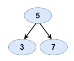
- Input: [5,3,7]
- Expected Output: true
- Justification: The left child of the root (3) is less than the root, and the right child of the root (7) is greater than the root. Hence, it’s a BST.
Example 2:
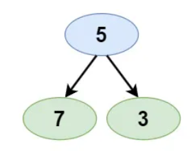
- Input: [5,7,3]
- Expected Output: false
- Justification: The left child of the root (7) is greater than the root, making it invalid.
Example 3:
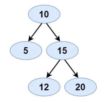
- Input: [10,5,15,null,null,12,20]
- Expected Output: true
- Justification: Each subtree of the binary tree is a valid binary search tree. So, a whole binary tree is a valid binary search tree.
Constraints:
- The number of nodes in the tree is in the range [1, 104].
- -2^31 <= Node.val <= 2^31- 1
Solution
In essence, to validate if a given binary tree is a binary search tree (BST), we employ a recursive approach that checks the validity of each node by comparing its value with a permissible range. This range is determined by the node’s ancestors, ensuring every node meets the BST property. Initially, the root node can take any value between negative infinity and positive infinity. As we traverse down the tree, we update this range based on the current node’s value.
Detailed Breakdown:
- Recursion:
- For each node in the binary tree, we validate its value against a permissible range. If the value does not lie within this range, the tree is not a BST.
- The range for any node is influenced by its ancestors, ensuring that every node, even those deep in the tree, satisfies the BST condition.
- Base Case:
- If the node we are inspecting is null (i.e., we’ve reached a leaf node), we return true since a null subtree is always a BST by definition.
- Recursive Step:
- Compare the node’s value against its permissible range. If it’s not within the range, return false.
- If it is within range, we recursively check the left and right children, but with updated permissible ranges.
- Implementation:
- Initially, the root node’s range is set to (-Infinity, +Infinity).
- For every left child, the upper limit of its permissible range is updated to the current node’s value. Similarly, for every right child, the lower limit is updated to the current node’s value.
Algorithm Walkthrough
For the tree [10,5,15,null,null,12,20]:
- Start with the root, range = (-Infinity, +Infinity)
- Node 10 is within the range.
- Move to the left child, range = (-Infinity, 10)
- Node 5 is within the range.
- Move to the right child of root, range = (10, +Infinity)
- Node 15 is within the range.
- Move to the left child of 15, range = (10, 15)
- Node 12 is within the range.
- Move to the right child of 15, range = (15, +Infinity)
- Node 20 is within the range.
- return true, as the next left node is null.
Code
1 | # class TreeNode: |
Complexity Analysis
- Time Complexity: O(n) - We traverse each node once.
- Space Complexity: O(h) - The space is determined by the height of the tree due to recursive calls. In the worst case (skewed tree), it’s O(n), while in the best case (balanced tree), it’s O(log n).
Construct Binary Tree from Preorder and Inorder Traversal
Problem Statement
Given the preorder and inorder traversal sequences of a binary tree, your task is to reconstruct this binary tree. Assume that the tree does not contain duplicate values.
Example Generation
Example 1:
- Input:
- Preorder: [1,2,4,5,3,6,7]
- Inorder: [4,2,5,1,6,3,7]
- Expected Output:
- Tree Representation: [1,2,3,4,5,6,7]
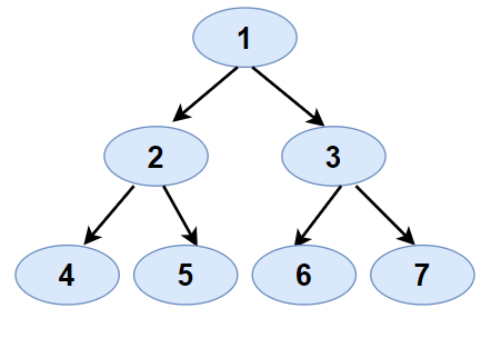
- Justification:
- The first value in preorder (1) is the root. In the inorder list, everything left of value 1 is the left subtree and everything on the right is the right subtree. Following this pattern recursively helps in reconstructing the binary tree.
Example 2:
- Input:
- Preorder: [8,5,9,7,1,12,2,4,11,3]
- Inorder: [9,5,1,7,2,12,8,4,3,11]
- Expected Output:
- Tree Representation: [8,5,4,9,7,11,1,12,2,null,3]
- Justification:
- Start with 8 (from preorder) as the root. Splitting at 8 in inorder, we find the left and right subtrees. Following this pattern recursively, we can construct the tree.
Example 3:
- Input:
- Preorder: [3,5,6,2,7,4,1,9,8]
- Inorder: [6,5,7,2,4,3,9,1,8]
- Expected Output:
- Tree Representation: [3,5,1,6,2,9,8,null,null,7,4]
- Justification:
- Following the same approach, using 3 as root from preorder, we split the inorder sequence into left and right subtrees and continue recursively.
Constraints:
1 <= preorder.length <= 3000inorder.length == preorder.length-3000 <= preorder[i], inorder[i] <= 3000preorderandinorderconsist of unique values.- Each value of
inorderalso appears inpreorder. preorderis guaranteed to be the preorder traversal of the tree.inorderis guaranteed to be the inorder traversal of the tree.
Solution
Reconstructing a binary tree from its preorder and inorder traversals involves recognizing the structure imposed by these traversal methods. The first element of the preorder traversal always gives us the root of the tree. Once we identify the root, its position in the inorder traversal divides the tree into its left and right subtrees. By harnessing this division recursively for both the left and the right subtrees, we can reconstruct the entire binary tree.
Detailed Steps:
- Start with Preorder’s Root: The first element in the preorder list is always the root of the tree.
- Find the Root in Inorder: Once we have the root from preorder, we find its position in the inorder sequence. This position divides the tree into its left and right subtrees.
- Recursion: Based on the root’s position in inorder, we can split both the preorder and inorder lists into two halves each - one for the left subtree and the other for the right subtree. We then recursively construct the left and right subtrees.
- Base Case: If the inorder sequence becomes empty, it indicates there’s no tree to construct, so we return
null.
This approach capitalizes on the properties of the preorder and inorder traversals to recursively reconstruct the tree.
Algorithm Walkthrough
Given Preorder: [1,2,4,5,3,6,7] and Inorder: [4,2,5,1,6,3,7]
- Take the first value from preorder (1) as the root.
- Find the position of 1 in inorder (position 4).
- Everything before position 4 in inorder is the left subtree, and everything after is the right subtree.
- Using the size of the left subtree (3 nodes), we take the next 3 values from preorder [2,4,5] for the left subtree and recursively repeat the process.
- Similarly, for the right subtree, we use the remaining values from preorder [3,6,7] and follow the same recursive approach.
Code
1 | # class TreeNode: |
Complexity Analysis
- Time Complexity: O(n). We are visiting each node once, and the look-up for the inorder index is constant time (due to HashMap or equivalent).
- Space Complexity: O(n). The space is majorly used for the hashmap and the recursive stack.
Clone Graph
Problem Statement
Given a reference of a node in a connected undirected graph, return a deep copy (clone) of the graph. Each node in the graph contains a value (int) and a list (List[Node]) of its neighbors.
Example 1:
Input:
1 | 1--2 |
Expected Output:
1 | 1--2 |
Explanation: The graph has four nodes with the following connections:
- Node
1is connected to nodes2and4. - Node
2is connected to nodes1and3. - Node
3is connected to nodes2and4. - Node
4is connected to nodes1and3.
Example 2:
Input:
1 | 1--2 |
Expected Output:
1 | 1--2 |
Explanation: The graph consists of five nodes with these connections:
- Node
1is connected to nodes2and5. - Node
2is connected to nodes1and3. - Node
3is connected to nodes2and4. - Node
4is connected to node3. - Node
5is connected to node1.
Example 3:
Input:
1 | 1--2 |
Expected Output:
1 | 1--2 |
Explanation: The graph has six nodes with the following connections:
- Node
1is connected to nodes2and4. - Node
2is connected to nodes1and3. - Node
3is connected to nodes2and6. - Node
4is connected to nodes1and5. - Node
5is connected to nodes4and6. - Node
6is connected to nodes3and5.
Constraints:
- The number of nodes in the graph is in the range
[0, 100]. 1 <= Node.val <= 100Node.valis unique for each node.- There are no repeated edges and no self-loops in the graph.
- The Graph is connected and all nodes can be visited starting from the given node.
Solution
To deep clone a given graph, the primary approach is to traverse the graph using Depth-First Search (DFS) and simultaneously create clones of the visited nodes. A hashmap (or dictionary) is utilized to track and associate original nodes with their respective clones, ensuring no duplications.
- Initialization: Create an empty hashmap to match the original nodes to their clones.
- DFS Traversal and Cloning: Traverse the graph with DFS. When encountering a node not in the hashmap, create its clone and map them in the hashmap. Recursively apply DFS for each of the node’s neighbors. After cloning a node and all its neighbors, associate the cloned node with the clones of its neighbors.
- Termination: Once DFS covers all nodes, return the cloned version of the starting node.
Algorithm Walkthrough (using Example 1):
For the input graph:
1 | 1--2 |
- Start with an empty hashmap
visited. - Begin DFS with node
1.- Node
1isn’t invisited. Clone it to get1'and map(1, 1')in the hashmap. - For each neighbor of node
1, apply DFS.- First with
2.- Node
2isn’t invisited. Clone to get2'and map(2, 2'). - Node
2‘s neighbors are1and3. Node1is visited, so link2'to1'. Move to3.- Node
3isn’t invisited. Clone to get3'and map(3, 3'). - Node
3has neighbors2and4. Node2is visited, so link3'to2'. Move to4.- Node
4isn’t invisited. Clone to get4'and map(4, 4'). - Node
4has neighbors1and3, both visited. Link4'to1'and3'.
- Node
- Node
- Node
- First with
- Node
- With DFS complete, return the clone of the starting node,
1'.
Code
1 | from collections import deque |
Complexity Analysis
- Time Complexity: O(N+M) where N is the number of nodes and M is the number of edges. Each node and edge is visited once.
- Space Complexity: O(N) as we are creating a clone for each node. Additionally, the recursion stack might use O(H) where H is the depth of the graph (in the worst case this would be O(N)).
House Robber II
Problem Statement
You are given an array representing the amount of money each house has. This array models a circle of houses, meaning that the first and last houses are adjacent. You are tasked with figuring out the maximum amount of money you can rob without alerting the neighbors.
The rule is: if you rob one house, you cannot rob its adjacent houses.
Examples
Example 1:
- Input: [4, 2, 3, 1]
- Expected Output: 7
- Justification: Rob the 1st and 3rd house, which gives 4 + 3 = 7.
Example 2:
- Input: [5, 1, 2, 5]
- Expected Output: 7
- Justification: Rob the 1st and 3rd house, which gives 5 + 2 = 7.
Example 3:
- Input: [1, 2, 3, 4, 5]
- Expected Output: 8
- Justification: Rob the 3rd and 5th house, which gives 3 + 5 = 8.
Constraints:
1 <= nums.length <= 1000 <= nums[i] <= 1000
Solution
The core idea of our algorithm is to split the circular house problem into two simpler linear problems and then solve each linear problem using a dynamic programming approach. Since the first and last houses in the circle are adjacent, we can’t rob them both. Thus, we consider two scenarios: robbing houses excluding the first one and robbing houses excluding the last one. For each scenario, we use a helper function that returns the maximum amount we can rob. This helper function utilizes dynamic programming to keep track of the cumulative robbery amounts, ensuring that no two consecutive houses are robbed. Finally, our solution is the maximum of the two scenarios.
Edge Cases Handling: Begin by checking for edge cases:
- If the input array is
nullor has a length of 0, return 0 since there are no houses to rob. - If there’s only one house, return its value.
- If there are two houses, return the maximum value of the two houses.
- If the input array is
Two Scenarios Handling: Due to the circular structure, handle two scenarios:
- Exclude the first house and compute for the rest.
- Exclude the last house and compute for the others.
Use a helper function to compute the maximum for each scenario.
Simple Robber Helper Function: This function calculates the maximum robbing amount for a linear set of houses using dynamic programming:
- Maintain two variables,
prevMaxandcurrMax, to keep track of the max amount robbed up to the previous and current house, respectively. - Iterate through each house in the given range (based on the scenario). At each house, decide whether to rob it (in which case you can’t rob the previous house) or skip it.
- For each house, update
currMaxbased on whether robbing the current house results in a larger amount than skipping it.
- Maintain two variables,
Return the Maximum: The main function concludes by returning the maximum value from the two scenarios.
Algorithm Walkthrough
Using the input [4, 2, 3, 1]:
Check for edge cases. Since the array has more than two houses, move to the next step.
Calculate the maximum amount that can be robbed for the two scenarios:
a. For the scenario excluding the last house (consider houses from index 0 to 2):
- Start with
prevMax = 0andcurrMax = 0. - For the first house (value 4),
currMaxbecomes 4. - For the second house (value 2),
currMaxremains 4 (because 4 > 2 + 0). - For the third house (value 3),
currMaxbecomes 7 (because 4 + 3 > 4). So, for this scenario, the maximum is 7.
b. For the scenario excluding the first house (consider houses from index 1 to 3):
- Start with
prevMax = 0andcurrMax = 0. - For the second house (value 2),
currMaxbecomes 2. - For the third house (value 3),
currMaxbecomes 3 (because 3 > 2). - For the fourth house (value 1),
currMaxremains 3 (because 3 > 1 + 2). So, for this scenario, the maximum is 3.
- Start with
The main function then returns the maximum of the two scenarios, which is 7 in this case.
Code
1 | class Solution: |
Complexity Analysis
Time Complexity: We are solving the house robber problem twice (once excluding the first house and once excluding the last house). Each run of the house robber problem has a time complexity of (O(n)), where (n) is the number of houses. Thus, our overall time complexity is (O(n)).
Space Complexity: We use a constant amount of space to store our previous and current max values. Hence, the space complexity is (O(1)).
Decode Ways
Problem Statement
You have given a string that consists only of digits. This string can be decoded into a set of alphabets where ‘1’ can be represented as ‘A’, ‘2’ as ‘B’, … , ‘26’ as ‘Z’. The task is to determine how many ways the given digit string can be decoded into alphabets.
Examples
- Input: “121”
- Expected Output: 3
- Justification: The string “121” can be decoded as “ABA”, “AU”, and “LA”.
- Input: “27”
- Expected Output: 1
- Justification: The string “27” can only be decoded as “BG”.
- Input: “110”
- Expected Output: 1
- Justification: The string “110” can only be decoded as “JA”.
Constraints:
1 <= s.length <= 100scontains only digits and may contain leading zero(s).
Solution
Our approach to solving this problem involves using dynamic programming to iteratively build the solution. Given a string of digits, we want to determine how many ways it can be decoded into alphabets. The key insight is that the number of ways to decode a string of length i is dependent on the number of ways to decode the previous two substrings of length i-1 and i-2. We’ll use two variables, prev and current, to store these values and update them as we loop through the string.
- Initialization: Begin by checking if the string is valid for decoding (e.g., it should not start with a ‘0’). If the string is invalid, return 0. Next, initialize two variables,
prevandcurrent, both set to 1.prevwill store the number of ways to decode the string of lengthi-2, andcurrentwill store the number of ways to decode the string of lengthi-1. - Iterate Through the String: Loop through the string from the second character to the end. For each character, compute the number of ways it can be decoded when combined with the previous character.
- Update Variables: For each character, evaluate the following conditions:
- If the current character and the previous character form a valid number between 10 and 26, they can be decoded together.
- If the current character is not ‘0’, it can be decoded individually. Use these conditions to update the
prevandcurrentvariables accordingly.
- Return the Result: Once the iteration completes, the
currentvariable will hold the total number of ways the entire string can be decoded. Return this value.
This dynamic programming approach is efficient because it computes the solution by using previously calculated results, and it avoids redundant calculations. By tracking and updating the number of ways to decode the current and previous substrings, the algorithm effectively builds the solution for the entire string.
Algorithm Walkthrough
Consider the input “121”:
- Initialize
prev = 1andcurrent = 1. - For the second character ‘2’:
- “12” can be decoded as “AB” or “L”.
- Update
prevandcurrentby swapping their values and settingcurrent += prev. - Now,
prev = 1andcurrent = 2.
- For the third character ‘1’:
- “21” can be decoded as “BA” or “U”.
- Again, update
prevandcurrent. - Now,
prev = 2andcurrent = 3.
- The final answer is 3, which is the value of
current.
Code
1 | class Solution: |
Complexity Analysis
- Time Complexity: O(N), where N is the length of the string. We loop through the string once.
- Space Complexity: O(1), as we only use a constant amount of space regardless of the input size.
Unique Paths
Problem Statement
Given a 2-dimensional grid of size m x n (where m is the number of rows and n is the number of columns), you need to find out the number of unique paths from the top-left corner to the bottom-right corner. The constraints are that you can only move either right or down at any point in time.
Examples
Example 1:
Input: 3, 3
Expected Output: 6
Justification:
The six possible paths are:
1. Right, Right, Down, Down
2. Right, Down, Right, Down
3. Right, Down, Down, Right
4. Down, Right, Right, Down
5. Down, Right, Down, Right
6. Down, Down, Right, Right
Example 2:
- Input: 3, 2
- Expected Output: 3
- Justification: The three possible paths are:
- Right, right, down
- Right, down, right
- Down, right, right
Example 3:
- Input: 2, 3
- Expected Output: 3
- Justification: The three possible paths are:
- Down, right, right
- Right, down, right
- Right, right, down
Solution
The unique paths problem can be approached using a dynamic programming solution. Essentially, the idea is to think of the grid as a graph where each cell is a node. Given we can only move right or down, the number of ways to reach a cell is the sum of the number of ways to reach the cell above it and the cell to its left. By breaking down the problem in this way, we can iteratively compute the number of paths to reach any cell, starting from the top-left and working our way to the bottom-right of the grid.
- Initialization:
- Create a 2-dimensional array
dpof sizem x ninitialized to zero. This array will store the number of unique paths to reach each cell.
- Create a 2-dimensional array
- Boundary Cases:
- All cells in the first row can only be reached by moving right from the top-left corner. So, the number of unique paths for all cells in the first row will be 1.
- Similarly, all cells in the first column can only be reached by moving downwards from the top-left corner. So, the number of unique paths for all cells in the first column will be 1.
- Filling the Table:
- For each remaining cell, the number of unique paths to that cell is the sum of the number of paths from the cell above it and the cell to the left of it. This is because we can only move right or down.
- Result:
- The bottom-right cell will contain the total number of unique paths from the top-left corner to the bottom-right corner.
Algorithm Walkthrough
Using the input from Example 1 (2, 2):
Initialize a 2x2 matrix
dpwith all zeros.1
20 0
0 0Fill the first row and first column with 1s.
1
21 1
1 0For cell
dp[1][1], add values from cell above (dp[0][1]) and cell to the left (dp[1][0]).1
21 1
1 2The bottom-right cell (
dp[1][1]) contains the number of unique paths: 2.
Constraints:
1 <= m, n <= 100
Code
1 | class Solution: |
Complexity Analysis
- Time Complexity: O(m * n) - We are processing each cell once.
- Space Complexity: O(m * n) - Due to the 2D dp array.
Word Break
Problem Statement
Given a non-empty string and a dictionary containing a list of non-empty words, determine if the string can be segmented into a space-separated sequence of one or more dictionary words. Each word in the dictionary can be reused multiple times.
Examples
Example 1:
- Input:
- String: “ilovecoding”
- Dictionary: [“i”, “love”, “coding”]
- Expected Output: True
- Justification: The string can be segmented as “i love coding”.
Example 2:
- Input:
- String: “helloworld”
- Dictionary: [“hello”, “world”, “hell”, “low”]
- Expected Output: True
- Justification: The string can be segmented as “hello world”.
Example 3:
- Input:
- String: “enjoylife”
- Dictionary: [“enj”, “life”, “joy”]
- Expected Output: False
- Justification: Despite having the words “enj” and “life” in the dictionary, we can’t segment the string into the space-separated dictionary words.
Constraints:
1 <= s.length <= 3001 <= wordDict.length <= 10001 <= wordDict[i].length <= 20sandwordDict[i]consist of only lowercase English letters.- All the strings of wordDict are unique.
Solution
Our algorithm’s primary objective is to determine whether the given string can be broken down into a sequence of words present in the dictionary. To achieve this, we use a dynamic programming approach, maintaining an array to keep track of the possibility of forming valid sequences up to every index of the string. The primary idea is to iterate through the string and, at each step, check all possible word endings at the current position. If a valid word is found, and the starting position of that word was marked as achievable, we mark the current position as achievable too.
- Initialization:
- Begin by initializing a boolean array
dpof sizen+1, wherenis the length of the string. This array will record whether the string can be segmented up to a certain index. We set the first element,dp[0], totruesince an empty string can always be segmented.
- Begin by initializing a boolean array
- Dynamic Programming:
- Iterate over the length of the string. For each index
i, verify every substring ending atiand see if it exists in the dictionary. - If a valid word is found and the starting position (denoted as
dp[j]) of the substring is true, setdp[i+1]to true. - Proceed in this manner until you reach the end of the string.
- Iterate over the length of the string. For each index
- Result:
- Once the iteration is complete, the value of
dp[n]will indicate if the entire string can be segmented into dictionary words or not.
- Once the iteration is complete, the value of
- Optimization:
- For faster lookups, convert the word dictionary into a set. This ensures constant time complexity when searching for words in the dictionary.
Algorithm Walkthrough
Given the string “helloworld” and dictionary [“hello”, “world”, “hell”, “low”]:
- Initialize
dpto[true, false, false, ..., false](length = 11 since “helloworld” has 10 characters). - For
i = 0, substring = “h”. It’s not in the dictionary, so move to next. - For
i = 1, substring = “he”, “h”. Neither is in the dictionary. - For
i = 4, substring = “hello”, which is in the dictionary anddp[0]is true. So, setdp[5]to true. - Continuing this, when we get to
i = 9, substring = “world” is in the dictionary, anddp[5]is true, so we setdp[10]to true. - Finally,
dp[10]is true, so “helloworld” can be segmented.
Code
1 | class Solution: |
Complexity Analysis
- Time Complexity: O(n^2) due to the two nested loops where we check all possible substrings.
- Space Complexity: O(n) for the DP array and the word set.
Lowest Common Ancestor of a Binary Search Tree
Problem Statement
Given a binary search tree (BST) and two of its nodes, find the node that is the lowest common ancestor (LCA) of the two given nodes. The LCA of two nodes is the node that lies in between the two nodes in terms of value and is the furthest from the root. In other words, it’s the deepest node where the two nodes diverge in the tree. Remember, in a BST, nodes have unique values.
Examples
Input:
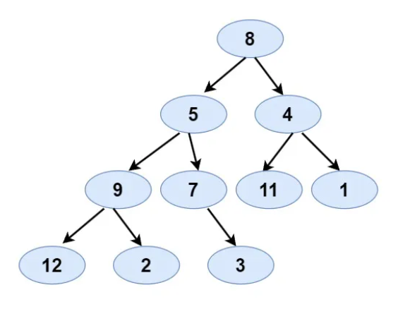
- BST: [6,2,8,0,4,7,9,null,null,3,5]
- Node 1: 2
- Node 2: 8
Expected Output: 6
- Justification: The nodes 2 and 8 are on the left and right children of node 6. Hence, node 6 is their LCA.
Input:
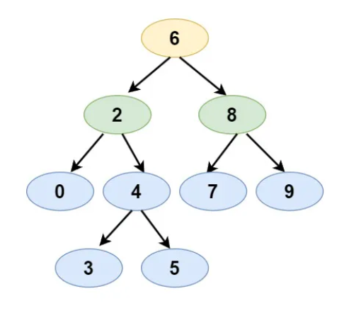
- BST: [6,2,8,0,4,7,9,null,null,3,5]
- Node 1: 0
- Node 2: 3
Expected Output: 2
- Justification: The nodes 0 and 3 are on the left and right children of node 2, which is the closest ancestor to these nodes.
Input:
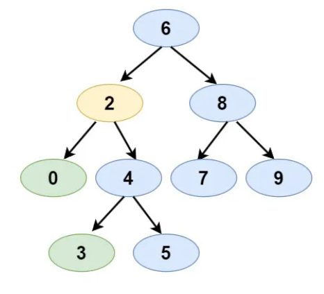
- BST: [6,2,8,0,4,7,9,null,null,3,5]
- Node 1: 4
- Node 2: 5
Expected Output: 4
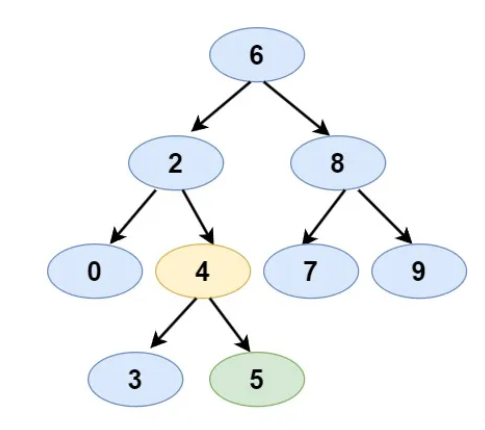
- Justification: Node 5 is the right child of node 4. Hence, the LCA is node 4 itself.
Constraints:
- The number of nodes in the tree is in the range [2, 105].
- -10^9 <=
Node.val<= 10^9 - All
Node.valare unique. p != qpandqwill exist in the BST.
Solution
The binary search tree property helps us find the solution without exploring the entire tree. Each node, starting from the root, provides a range based on its value that can determine where the two nodes are located.
- Starting at the Root: Begin at the root of the BST.
- Determining Direction: If the values of both nodes are greater than the current root node’s value, then the LCA must be in the right subtree. If the values are both less, then the LCA is in the left subtree.
- Divergence Point: If one node’s value is less than the root’s value and the other node’s value is greater (or if one of them matches the root’s value), then the current root is the LCA, since the path to reach both nodes diverges from here.
- Iterative Search: Repeat the process iteratively on the selected subtree (either left or right) until you find the LCA.
Algorithm Walkthrough
Using the first example input:
- BST: [6,2,8,0,4,7,9,null,null,3,5]
- Node 1: 2
- Node 2: 8
Steps:
- Start at root which is 6.
- Both 2 and 8 are on different sides of 6 (2 on the left and 8 on the right).
- Therefore, 6 is the lowest common ancestor.
Code
1 | # class TreeNode: |
Complexity Analysis
The algorithm traverses the BST in a single path, either going left or right, but never both. Therefore:
- Time Complexity: O(h), where h is the height of the BST.
- pace Complexity: O(1) since we only used a constant amount of space.
Longest Consecutive Sequence
Problem Statement
Given an unsorted array of integers, find the length of the longest consecutive sequence of numbers in it. A consecutive sequence means the numbers in the sequence are contiguous without any gaps. For instance, 1, 2, 3, 4 is a consecutive sequence, but 1, 3, 4, 5 is not.
Examples
- Input: [10, 11, 14, 12, 13]
- Output: 5
- Justification: The entire array forms a consecutive sequence from 10 to 14.
- Input: [3, 6, 4, 100, 101, 102]
- Output: 3
- Justification: There are two consecutive sequences, [3, 4] and [100,101,102]. The latter has a maximum length of 3.
- Input: [4, 3, 6, 2, 5, 8, 4, 7, 0, 1]
- Output: 9
- Justification: The longest consecutive sequences here are [0, 1, 2,, 3, 4, 5, 6, 7, 8].
- Input: [7, 8, 10, 11, 15]
- Output: 2
- Justification: The longest consecutive sequences here are [7,8] and [10,11], both of length 2.
Constraints:
- 0 <= nums.length <= 105
- -10^9 <= nums[i] <= 10^9
Solution
To solve this problem, the key observation is that if n is part of a consecutive sequence, then n+1 and n-1 must also be in that sequence.
- HashSet: Begin by inserting all elements of the array into a HashSet. The reason for using a HashSet is to ensure O(1) time complexity during look-up operations.
- Initial Scan: Iterate through each element of the array. For every number, check if it’s the starting point of a possible sequence. This can be determined by checking if
n-1exists in the HashSet. If not, then it meansnis the start of a sequence. - Building Sequences: For each starting number identified in step 2, keep checking if
n+1,n+2… exist in the HashSet. For each present number, increase the length of the sequence and move to the next number. - Result: Store the length of each sequence found in step 3. The answer will be the longest of all sequences identified.
Algorithm Walkthrough
Given the input: [3, 6, 4, 100, 101, 102]
- Initialize an empty HashSet and populate it with all numbers from the input.
- Start with the first number, 3. Since 2 (which is 3-1) is not in the HashSet, we recognize 3 as the starting of a sequence.
- Check for 4. It’s there. Move to 5. It’s not there. So, the sequence is [3,4] with a length of 2.
- Next, take 6. 5 is not there, so 6 might be the start of a new sequence. However, 7 isn’t in the HashSet. So, the sequence is just [6].
- For 100, 99 isn’t there, so 100 is a starting point.
- Check for 101. It’s there. Check for 102. It’s there. Check for 103. It’s not there. The sequence is [100,101,102] with a length of 3.
- The algorithm returns 3, which is the length of the longest sequence.
Code
1 | class Solution: |
Complexity Analysis
- Time Complexity: O(n). Although it seems that the while loop runs for each number, it only runs for the numbers that are the starting points of sequences. So, in total, each number is processed only once.
- Space Complexity: O(n). The space used by our set.
Meeting Rooms II
Problem Statement
Given a list of time intervals during which meetings are scheduled, determine the minimum number of meeting rooms that are required to ensure that none of the meetings overlap in time.
Examples
- Example 1:
- Input:
[[10, 15], [20, 25], [30, 35]] - Expected Output:
1 - Justification: There are no overlapping intervals in the given list. So, only 1 meeting room is enough for all the meetings.
- Input:
- Example 2:
- Input:
[[10, 20], [15, 25], [24, 30]] - Expected Output:
2 - Justification: The first and second intervals overlap, and the second and third intervals overlap as well. So, we need 2 rooms.
- Input:
- Example 3:
- Input:
[[10, 20], [20, 30]] - Expected Output:
1 - Justification: The end time of the first meeting is the same as the start time of the second meeting. So, one meeting can be scheduled right after the other in the same room.
- Input:
Constraints:
- 1 <= intervals.length <= 104
- 0 <= starti < endi <= 106
Solution
To determine the minimum number of rooms required to host the meetings without any time overlap, our approach first involves sorting all meeting intervals based on their start times. This sorting allows us to sequentially evaluate meetings in the order they start. We then utilize a priority queue (min-heap) to keep track of end times of the meetings currently taking place. This queue helps in efficiently determining the earliest ending meeting. By sequentially examining each meeting and comparing its start time to the earliest ending time from the heap, we can decide if a new room is needed or if an existing room can be reused.
- Sorting: Begin by sorting all intervals based on their start times. This enables us to sequentially check for overlapping intervals.
- Priority Queue: A priority queue (min-heap) is used to monitor end times of meetings that are currently in session. If the start time of the next meeting is less than the smallest end time (i.e., the top of the priority queue), it indicates we require another room.
- Reusing Rooms: Once we have checked a meeting and it doesn’t overlap with the smallest end time, this means that the meeting room used by the meeting with the smallest end time can be reassigned. Therefore, we remove the earliest ending meeting from the priority queue.
- Counting Rooms: At any given time, the size of the priority queue reflects the number of rooms in use. This can be used to deduce the minimum number of rooms needed up to that point.
Algorithm Walkthrough
Given an input [[10, 20], [15, 30], [25, 40]]:
- First, sort the intervals:
[[10, 20], [15, 30], [25, 40]](in this case, the intervals are already sorted). - Initialize a priority queue. Add the end time of the first meeting to the queue.
- For the next interval
[15, 30], the start time 15 is less than the top of the queue (i.e., 20). Hence, we need another room. Add 30 to the priority queue. - For the next interval
[25, 40], the start time 25 is greater than the top of the queue (i.e., 20). So, we can use the room which will be free at time 20. Remove 20 from the queue and add 40. - The size of the priority queue at the end is 2, indicating 2 rooms are required.
Code
1 | import heapq |
Complexity Analysis
- Time Complexity: The time complexity of our algorithm is (O(N \log N)), where (N) is the number of intervals. This is because we’re sorting the intervals once and then using priority queues to process them.
- Space Complexity: The space complexity is (O(N)) as we’re storing all intervals in the worst case.
Encode and Decode Strings
Problem Statement
Given a list of strings, your task is to develop two functions: one that encodes the list of strings into a single string, and another that decodes the resulting single string back into the original list of strings. It is crucial that the decoded list is identical to the original one.
It is given that you can use any encoding technique to encode list of string into the single string.
Examples
- Example 1:
- Input: [“apple”, “banana”]
- Expected Output: [“apple”, “banana”]
- Justification: When we encode the input strings [“apple”, “banana”], we get a single encoded string. Decoding this encoded string should give us the original list [“apple”, “banana”].
- Example 2:
- Input: [“sun”, “moon”, “stars”]
- Expected Output: [“sun”, “moon”, “stars”]
- Justification: After encoding the input list, decoding it should bring back the original list.
- Example 3:
- Input: [“Hello123”, “&*^%”]
- Expected Output: [“Hello123”, “&*^%”]
- Justification: Regardless of the content of the string (special characters, numbers, etc.), decoding the encoded list should reproduce the original list.
Constraints:
1 <= strs.length <= 2000 <= strs[i].length <= 200strs[i]contains any possible characters out of 256 valid ASCII characters.
Solution
Our approach will utilize a delimiter that doesn’t appear in the input strings. For the sake of simplicity, we can choose a character like #. If # is possible in the input, we can use multiple characters like ## to reduce the chance it appears in the input.
- Encoding:
- For each string in the list, we append it to the encoded string.
- After appending the string, we add the delimiter
##. - Continue this for all the strings in the list.
- Decoding:
- We split the encoded string using our delimiter
##. - This will give us a list of strings which is our original list.
- We split the encoded string using our delimiter
- Handling Edge Cases:
- If
##can be part of the input strings, then our approach will fail. To handle such cases, we can prefix each string with its length followed by a special character, like|, before the actual string. This way, during decoding, we can use the length to identify the end of one string and the beginning of the next.
- If
Algorithm Walkthrough
Let’s walk through the algorithm using the input [“apple”, “banana##cherry”]:
- During encoding:
- “apple” becomes “5|apple##”
- “banana##cherry” becomes “15|banana##cherry##”
- The final encoded string is “5|apple##15|banana##cherry##”
- During decoding:
- Read the first character, which is
5. It tells us the next 5 characters form the first string “apple”. - The next character
#is part of our delimiter, so we skip two characters. - Next, read the number
15, which tells us the next 15 characters form the string “banana##cherry”. - Finally, we reach the end of our encoded string.
- Read the first character, which is
Code
1 | class Solution: |
Complexity Analysis
- Time Complexity:
- For encoding, it is (O(n)), where (n) is the combined length of all the strings in the list because we iterate over each character once.
- For decoding, it’s also (O(n)) for the same reason.
- Space Complexity: (O(n)) as we store the encoded version of the string, and its length is proportional to the combined length of all the strings in the list.
Number of Connected Components in an Undirected Graph
Problem Statement
Given an undirected graph represented by ‘n’ nodes labeled from 0 to n-1 and a list of undirected edges (each edge is a pair of nodes), determine the number of connected components in the graph. A connected component is a group of nodes that are directly or indirectly linked to each other through the edges.
Examples
- Example 1
- Input:
n = 5,edges = [[0,1], [2,3], [3,4]]
- Input:
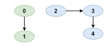
- Expected Output:
2 - Justification: Two components are:
0-1, and2-3-4.
- Example 2
- Input:
n = 4,edges = [[0,1], [1,2], [2,3]]
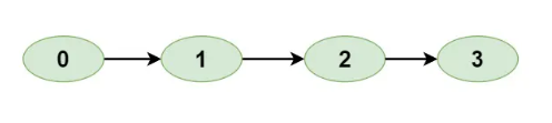
- Expected Output:
1 - Justification: All the nodes are connected in a single chain:
0-1-2-3.
- Example 3
- Input:
n = 3,edges = [[0,1]]
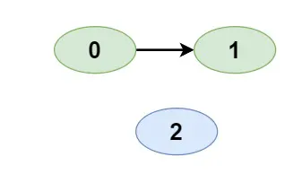
- Expected Output:
2 - Justification: Two connected components exist:
0-1and an isolated node2.
Constraints:
1 <= n <= 20001 <= edges.length <= 5000edges[i].length == 2- 0 <= ai <= bi < n
- ai != bi
- There are no repeated edges.
Solution
We will use the Union-Find (also known as Disjoint Set Union, DSU) data structure to solve this problem. This approach is efficient in identifying and merging different sets:
- Initialization:
- Create an array
parentof sizenwhereparent[i] = i. This array will keep track of the parent of each node. Initially, each node is its own parent. - Count the number of separate components. Initially, the count is
nsince every node is a separate component.
- Create an array
- Union Operation:
- For each edge
(u, v), find the parent ofuand the parent ofv. - If the parents are different, then
uandvbelong to different components. So, we merge them by assigning one’s parent to the other and reduce the component count by 1.
- For each edge
- Find Operation:
- This operation determines the parent of a node. If a node’s parent is itself, return the node. Otherwise, recursively find the parent of its parent. To optimize the search in future look-ups, we can apply path compression by updating the parent of the current node to its root during the recursion.
- Result:
- After processing all edges, the component count will represent the number of connected components.
Algorithm Walkthrough
Using the input n = 5 and edges = [[0,1], [2,3], [3,4]]:
- Initialize
parent = [0, 1, 2, 3, 4]andcount = 5. - Process edge
[0,1]:- Parent of 0 is 0.
- Parent of 1 is 1.
- They have different parents. Merge them by setting parent of 1 to 0 and reduce count to 4.
- Process edge
[2,3]:- Parent of 2 is 2.
- Parent of 3 is 3.
- Merge them by setting parent of 3 to 2. Reduce count to 3.
- Process edge
[3,4]:- Parent of 3 is 2 (from previous merge).
- Parent of 4 is 4.
- Merge them by setting parent of 4 to 2. Reduce count to 2.
- Final count is 2.
Code
1 | class Solution: |
Complexity Analysis
- Time Complexity: The union operation is almost O(1) with path compression. So, for
Eedges, the time complexity is approximately O(E). - Space Complexity: O(N) due to the
parentarray.
Graph Valid Tree
Problem Statement
Given a number n, which indicates the number of nodes numbered from 0 to n-1, and a list of undirected edges for the graph, determine if the graph is a valid tree.
A graph qualifies as a valid tree if it meets the following criteria:
- It has no cycles.
- It is fully connected.
Examples
- Example 1:
- Input: n = 5, edges = [[0,1],[0,2],[0,3],[1,4]]
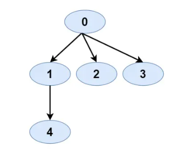
- Expected Output: true
- Justification: There are no cycles in the graph, and all nodes are connected, forming a valid tree.
- Example 2:
- Input: n = 4, edges = [[0,1],[1,2],[2,3],[3,0]]]]
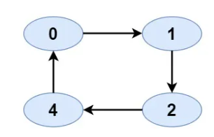
- Expected Output: false
- Justification: There is a cycle in the graph (0-1-2-3-0), thus it’s not a valid tree.
- Example 3:
- Input: n = 5, edges = [[0,1],[1,2],[2,3]]
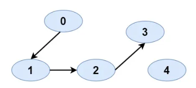
- Expected Output: false
- Justification: TNode 4 is not connected to any other node, making the graph not fully connected.
Constraints:
1 <= n <= 20000 <= edges.length <= 5000edges[i].length == 2- 0 <= ai <= bi < n
- ai != bi
- There are no self-loops or repeated edges.
Solution
To determine if a given undirected graph forms a valid tree, we must ensure two key conditions are met:
- The graph should not have any cycles.
- The graph should be fully connected (i.e., all nodes are reachable from any other node).
To verify these conditions, we can adopt the following approach:
- Initialization: Construct an adjacency list for the graph. Initialize a set (or an array) to keep track of visited nodes.
- DFS for Cycle Check: Use Depth First Search (DFS) to explore the graph. During this traversal, if we ever try to revisit a node we’ve previously visited (excluding the parent node), it indicates the presence of a cycle.
- Connectivity Check: After ensuring there are no cycles, we need to ensure that the graph is fully connected. This can be done by verifying that the number of unique nodes visited during our DFS equals the total number of nodes.
- Return Result: If both checks pass, then it’s a valid tree and we return true. Otherwise, return false.
Algorithm Walkthrough
Using the input from Example 1:
1 | n = 5 |
Start with the adjacency list:
1
2
3
4
50 -> [1, 2, 3]
1 -> [0, 4]
2 -> [0]
3 -> [0]
4 -> [1]Start DFS from node 0. Mark node 0 as visited.
Move to node 1 (from node 0). Mark node 1 as visited.
From node 1, visit node 4. Mark node 4 as visited.
Backtrack to node 1, and backtrack again to node 0.
From node 0, visit node 2. Mark node 2 as visited.
From node 0, visit node 3. Mark node 3 as visited.
At the end of DFS, we’ve visited all nodes and found no cycles.
Since we visited all nodes, the graph is fully connected.
Hence, the graph is a valid tree.
Code
1 | from collections import defaultdict |
Complexity Analysis
- Time Complexity: The algorithm visits each node and edge once, so its time complexity is ( O(n + e) ), where ( n ) is the number of nodes and ( e ) is the number of edges.
- Space Complexity: We are using a graph and visited set, so the space complexity is ( O(n + e) ).
Implement Trie (Prefix Tree)
Problem Statement
Design and implement a Trie (also known as a Prefix Tree). A trie is a tree-like data structure that stores a dynamic set of strings, and is particularly useful for searching for words with a given prefix.
Implement the Solution class:
Solution()Initializes the object.void insert(word)Insertswordinto the trie, making it available for future searches.bool search(word)Checks if the word exists in the trie.bool startsWith(word)Checks if any word in the trie starts with the given prefix.
Examples
- Example 1:
- Input:
- Trie operations:
["Trie", "insert", "search", "startsWith"] - Arguments:
[[], ["apple"], ["apple"], ["app"]]
- Trie operations:
- Expected Output:
[-1, -1, 1, 1] - Justification: After inserting “apple”, “apple” exists in the Trie. There is also a word that starts with “app”, which is “apple”.
- Input:
- Example 2:
- Input:
- Trie operations:
["Trie", "insert", "search", "startsWith", "search"] - Arguments:
[[], ["banana"], ["apple"], ["ban"], ["banana"]]
- Trie operations:
- Expected Output:
[-1, -1, 0, 1, 1] - Justification: After inserting “banana”, “apple” does not exist in the Trie but a word that starts with “ban”, which is “banana”, does exist.
- Input:
- Example 3:
- Input:
- Trie operations:
["Trie", "insert", "search", "search", "startsWith"] - Arguments:
[[], ["grape"], ["grape"], ["grap"], ["gr"]]
- Trie operations:
- Expected Output:
[-1, -1, 1, 1, 1] - Justification: After inserting “grape”, “grape” exists in the Trie. There are words that start with “grap” and “gr”, which is “grape”.
- Input:
Constraints:
1 <= word.length, prefix.length <= 2000wordand prefixconsist only of lowercase English letters.- At most 3 * 104 calls in total will be made to insert, search, and startsWith.
Solution
The trie is represented as a tree, where each node contains an array of pointers (or references) to its children and a boolean flag indicating if the current node marks the end of a word. When inserting or searching for a word, we start at the root node and navigate through the tree character by character until we either finish the operation or determine the word doesn’t exist in the trie.
Now, let’s break down the operations:
- Insert:
- We begin at the root node.
- For every character in the word, check if there’s a child node for it.
- If the child node doesn’t exist, we create it.
- Navigate to the child node and repeat the process for the next character.
- Once the end of the word is reached, mark the current node as an endpoint of a word.
- Search:
- Starting at the root, traverse the trie character by character.
- For every character in the word, check if there’s a child node for it.
- If at any point there isn’t a child node for the character, the word doesn’t exist in the trie.
- If we can traverse the entire word and the last node is marked as an endpoint, the word exists in the trie.
- StartsWith:
- The operation is similar to the search, but we don’t need the last node to be an endpoint.
- If we can traverse the prefix without any missing nodes, there exists a word in the trie that starts with the given prefix.
Algorithm Walkthrough
Using Example 1:
["Trie", "insert", "search", "startsWith"][[], ["apple"], ["apple"], ["app"]]
- Create an empty Trie.
- Insert “apple”.
- Start from the root. For ‘a’, move to the child node or create one if it doesn’t exist.
- Move to ‘p’, then the next ‘p’, followed by ‘l’ and finally ‘e’. Mark ‘e’ as the end of a word.
- Search for “apple”.
- Start from the root and traverse nodes ‘a’ -> ‘p’ -> ‘p’ -> ‘l’ -> ‘e’. Since ‘e’ is marked as the end of a word, return true.
- Check if a word starts with “app”.
- Traverse nodes for ‘a’ -> ‘p’ -> ‘p’. All nodes exist, so return true.
Code
1 | # class TrieNode: |
Complexity Analysis
- Time Complexity:
- Insert: (O(m)), where (m) is the key length.
- Search and StartsWith: (O(m)) in the worst case scenario.
- Space Complexity: (O(n \times m)), where (n) is the number of inserted keys and (m) is the average key length.
Design Add and Search Words Data Structure
Problem Statement
Design a data structure that supports the addition of new words and the ability to check if a string matches any previously added word.
Implement the Solution class:
Solution()Initializes the object.void addWord(word)Insertswordinto the data structure, making it available for future searches.bool search(word)Checks if there is any word in the data structure that matchesword. The method returnstrueif such a match exists, otherwise returnsfalse.
Note: In the search query word, the character '.' can represent any single letter, effectively serving as a wildcard character.
Examples
Example 1:
Input:
1
2["Solution", "addWord", "addWord", "search", "search"]
[[], ["apple"], ["banana"], ["apple"], ["....."]]Expected Output:
1
[-1, -1, -1, 1, 1]
Justification: After adding the words “apple” and “banana”, searching for “apple” will return
truesince “apple” is in the data structure. Searching for “…..” will also returntrueas both “apple” and “banana” match the pattern.
Example 2:
Input:
1
2["Solution", "addWord", "addWord", "search", "search"]
[[], ["cat"], ["dog"], ["c.t"], ["d..g"]]Expected Output:
1
[-1, -1, -1, 1, 0]
Justification: “c.t” matches “cat” and “d..g” doesn’t matches “dog”.
Example 3:
Input:
1
2["Solution", "addWord", "search", "search"]
[[], ["hello"], ["h.llo"], ["h...o"]]Expected Output:
1
[-1, -1, 1, 0]
Justification: “h.llo” and “h…o” both match “hello”.
Constraints:
1 <= word.length <= 25wordinaddWordconsists of lowercase English letters.wordinsearchconsist of ‘.’ or lowercase English letters.- There will be at most 2 dots in word for search queries.
- At most 104 calls will be made to addWord and search.
Solution
The crux of the problem lies in efficiently inserting words and then searching for them, even if the query includes wildcards. To solve this, we utilize the trie (prefix tree) data structure. A trie is a tree-like structure that’s useful for storing a dynamic set of strings, especially when the dataset involves large numbers of queries on prefixes of strings. Each node of the trie can represent a character of a word, and the path from the root node to any node represents the word stored up to that point. The key operation for the wildcard is a recursive search, which allows us to explore multiple paths in the trie when we encounter the wildcard character.
1. Trie Data Structure: Every node of the trie contains multiple child nodes (one for each character of the alphabet). We start with a root node that represents an empty string. Each level of the trie represents the next character of a word.
2. Adding a Word: To insert a word into our trie, we begin at the root and traverse down the trie based on the characters in the word. If a particular character doesn’t have a corresponding child node in the current node, we create a new child node for that character. Once we’ve processed every character of the word, we mark the final node as the end of a valid word.
3. Searching: Searching for a word is similar to inserting, but with an additional consideration for the wildcard character (‘.’). If we encounter a ‘.’, we must consider all child nodes of the current node and recursively continue our search from each of them. If any of the paths result in a match, we return true. If we reach the end of a word without encountering any mismatches or premature ends, we’ve found a valid word in our trie.
This trie-based approach ensures efficient operations for both inserting and searching for words. In cases without wildcards, the search operation can be performed in linear time relative to the word’s length. However, with wildcards, the time complexity might increase, but the trie structure still ensures that we do this efficiently.
Algorithm Walkthrough
Given the word “apple” to insert and then search for “…..”:
- Start at the root node.
- For inserting “apple”:
- At ‘a’, move down or create a node if it doesn’t exist.
- At ‘p’, move down or create.
- Do the same for the next ‘p’, ‘l’, and ‘e’.
- Mark the last node (for ‘e’) as the end of a word.
- For searching “…..”:
- At the first ‘.’, check all child nodes and continue.
- Repeat for each ‘.’.
- If any path leads to a node that represents the end of a word, return
true.
Code
1 | # class TrieNode: |
Complexity Analysis
- Time Complexity:
- Insertion (addWord): O(n), where n is the length of the word. This is because each insertion operation runs in linear time with respect to the length of the word.
- Search: O(n * m) in the worst case, where n is the length of the word and m is the total number of nodes in the Trie. This happens when the search word contains dots (‘.’). However, for words without dots, the search is O(n).
- Space Complexity: O(m n), where m is the total number of Trie nodes and n is the average number of characters in the words. Each Trie node has up to 26 children (for each letter of the alphabet). In the worst case, when no nodes are shared, the space complexity is O(m n).