25. Pattern Union Find

Grokking Interview Pattern Interview

Word count: 5.9kReading time: 36 min

 2024/05/25 

Introduction to Union Find Pattern

Union Find, also known as Disjoint Set Union (DSU), is a data structure that keeps track of a partition of a set into disjoint subsets (meaning no set overlaps with another). It provides two primary operations: find, which determines which subset a particular element is in, and union, which merges two subsets into a single subset. This pattern is particularly useful for problems where we need to find whether 2 elements belong to the same group or need to solve connectivity-related problems in a graph or tree.

Core Operations of Union-Find (Disjoint Set Union - DSU):

Find: Determine which set a particular element belongs to. This can be used for determining if two elements are in the same set.
Union: Merge two sets together. This operation is used when there is a relationship between two elements, indicating they should be in the same set.

Union-Find: A Story of Connections

Imagine a social network where everyone is initially a single user with no friends. The moment two users become friends, they form a group. If a user befriends someone from another group, the two groups merge into a larger friend circle. Union-Find helps track these friendships and circles.

How DSU Work?

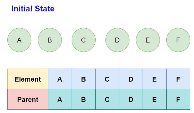
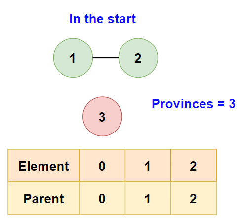
Initial State: Everyone is in their own separate group. Think of each person as their own little island.
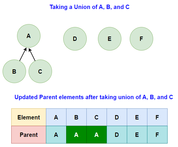
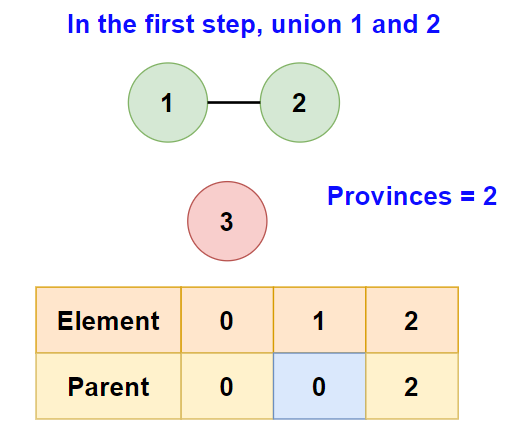
Making Connections (Union): When two people shake hands, they now belong to the same group. If they were already in groups, their entire groups merge.
Checking Connections (Find): Want to know if two people are connected? Union-Find can check if they’re in the same group.

How DSU is Implemented?

Parents Array: Each element has a parent. In the beginning, each element is their own parent.
Find Operation: Follows the chain of parents until it reaches the root parent, which represents the group.
Union Operation: Connects two groups by setting the parent of one group’s root to the other group’s root.

Operations on Disjoint Set Data Structures

1. Creating Disjoint Sets:

Each element points to a parent.
Initially, each element is its own parent, forming n disjoint sets.
A “root” element is one that points to itself, identifying the set’s representative.

1 2	# Initialize 'n' elements where each element is its own parent. parent = [i for i in range(n)] # 'n' is the number of elements

2. Find Operation:

The Find operation determines which set a particular element belongs to. This can be used to determine if two elements are in the same set.

In the below code:

parent is an array where parent[i] is the parent of i.
If parent[i] == i, then i is the root of the set and hence the representative.
The find function follows the chain of parents for i until it reaches the root.

def find(i):
    # If the element is its own parent, it's the representative of its set.
    if parent[i] == i:
        return i
    # Otherwise, recursively find the representative of the set.
    else:
        return find(parent[i])

Above function recursively traverses the parent array until it finds a node that is the parent of itself.

3. Union Operation:

The Union operation merges two disjoint sets. It takes two elements as input, finds the representatives of their sets using the Find operation, and finally merges the two sets.

def union(i, j):
    # Find the representatives of the two sets.
    irep = find(i)
    jrep = find(j)
    
    # If they are already in the same set, return.
    if irep == jrep:
        return
    
    # Make the representative of the first set point to the representative of the second set.
    parent[irep] = jrep

Above function merges two sets by making the representative of one set the parent of the other.

Now, we need to optimize the find() and union() methods.

Optimizations

Here are various methods for optimally perform operations on disjoint set.

1. Path Compression:

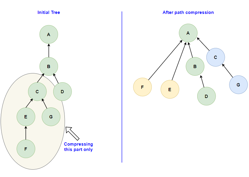
This optimization is applied during the Find operation. The idea behind path compression is to flatten the structure of the tree, making each member of the set point directly to the set’s representative. This ensures that subsequent Find operations are faster and more efficient. When an element’s representative is found using the Find operation, the element’s parent is updated to directly reference the representative, thereby compressing the path.

def find(i):
    # If i is the parent of itself
    if Parent[i] == i:
        # Then i is the representative of its set
        return i
    else:
        # Recursively find the representative of the set that i belongs to
        result = find(Parent[i])
        
        # Path Compression: Directly connect i to the representative of its set
        Parent[i] = result
        
        # Return the representative
        return result

This modified Find operation ensures that every node directly points to the representative of the set, and it makes it easy to find the representative of any two elements.

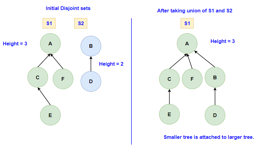
2. Union by Rank:

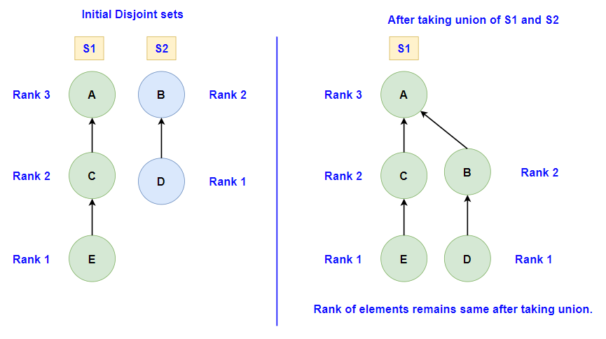
This optimization focuses on keeping the tree balanced during the Union operation. When two sets are merged, the tree with a smaller rank (or depth) is attached to the root of the tree with a larger rank. This ensures that the tree remains relatively flat, optimizing future operations. If both trees have the same rank, the rank of one of them is incremented by one, and the other tree is attached to it.

def unionbyrank(i, j):
    # Find the representatives of the two sets.
    irep = find(i)
    jrep = find(j)
    
    # If they are already in the same set, return.
    if irep == jrep:
        return
    
    # Attach the tree with a smaller rank under the tree with a larger rank.
    if rank[irep] < rank[jrep]:
        parent[irep] = jrep
    elif rank[irep] > rank[jrep]:
        parent[jrep] = irep
    # If both trees have the same rank, increase the rank of one tree by 1.
    else:
        parent[irep] = jrep
        rank[jrep] += 1

This function uses the rank array to decide which tree gets attached under which tree.

3. Union by Size:

Similar in spirit to Union by Rank, this optimization considers the size (or number of nodes) of the trees when merging them. The primary goal is to ensure that the smaller tree (in terms of nodes) is always attached to the larger tree. This approach helps in maintaining a balanced tree structure, ensuring that operations on the data structure remain efficient.

def unionbysize(i, j):
    # Find the representatives of the two sets.
    irep = find(i)
    jrep = find(j)
    
    # If they are already in the same set, return.
    if irep == jrep:
        return
    
    # Attach the smaller tree under the larger tree.
    if size[irep] < size[jrep]:
        parent[irep] = jrep
        size[jrep] += size[irep]
    else:
        parent[jrep] = irep
        size[irep] += size[jrep]

This function uses the size array to ensure that the tree with fewer nodes is added under the tree with more nodes.

Example

Here’s a complete implementation of the disjoint set with path compression and union by rank:

# Python3 program to implement Disjoint Set Data Structure.

class Solution:
    def __init__(self, n):
        # Constructor: Initialize sets of n items.
        # rank: Store the depth of trees (used for union by rank).
        self.rank = [1] * n
        # parent: Store the parent of each item. Initially, every item is its own parent.
        self.parent = [i for i in range(n)]

    def find(self, x):
        # If x is not its own parent, then it's not the representative of its set.
        if self.parent[x] != x:
            # Path Compression: Connect x directly to its set's representative.
            self.parent[x] = self.find(self.parent[x])
        # Return the representative of the set.
        return self.parent[x]

    def Union(self, x, y):
        # Find the representatives (or the root nodes) for x and y.
        xset = self.find(x)
        yset = self.find(y)

        # If x and y are already in the same set, return.
        if xset == yset:
            return

        # Union by Rank:
        # Attach the tree with a smaller rank under the root of the tree with a larger rank.
        if self.rank[xset] < self.rank[yset]:
            self.parent[xset] = yset
        elif self.rank[xset] > self.rank[yset]:
            self.parent[yset] = xset
        # If ranks are the same, choose one tree and increment its rank.
        else:
            self.parent[yset] = xset
            self.rank[xset] += 1

# Driver code
if __name__ == "__main__":
    # Create a disjoint set data structure with 5 elements.
    obj = Solution(5)
    # Merge sets that contain 0 and 2.
    obj.Union(0, 2)
    # Merge sets that contain 4 and 2.
    obj.Union(4, 2)
    # Merge sets that contain 3 and 1.
    obj.Union(3, 1)
    # Check if 4 and 0 are in the same set.
    if obj.find(4) == obj.find(0):
        print('Yes')
    else:
        print('No')
    # Check if 1 and 0 are in the same set.
    if obj.find(1) == obj.find(0):
        print('Yes')
    else:
        print('No')

Pros and Cons of DSU

Pros:
- Efficiency: Provides near constant time operations for union and find operations, making it highly efficient.
- Simplicity: Once set up, it’s straightforward to use for solving problems related to disjoint sets.
Cons:
- Space Overhead: Requires additional space to store the parent and rank of each element.
- Initial Setup: Requires initial setup to create and initialize the data structure.

Why Choose Union-Find Over BFS/DFS?

You can solve similar problems using the Breadth-First Search (BFS) and Depth-First Search (DFS) algorithms, but the Union Find algorithm provides the optimal solution over them. For problems related to connectivity checks and component identification, Union-Find is often more efficient than BFS/DFS.

Time Complexity:
- BFS/DFS: For BFS and DFS, the time complexity is O(V + E) where V is the number of vertices and E is the number of edges. This can be quite slow for large graphs.
- Union-Find: With path compression and union by rank, the amortized time complexity for union and find operations can be approximated as O(a(n)), where a(n) is the inverse Ackermann function. This function grows very slowly, making Union-Find operations almost constant time in practice.

Let’s jump onto our first problem and apply the Union Find pattern.

Redundant Connection

684. Redundant Connection Design Gurus

Problem Statement

Given an undirected graph containing 1 to n nodes. The graph is represented by a 2D array of edges, where edges[i] = [ai, bi], represents an edge between ai, and bi.

Identify one edge that, if removed, will turn the graph into a tree.

A tree is a graph that is connected and has no cycles.

Assume that the graph is always reducible to a tree by removing just one edge.

If there are multiple answers, return the edge that occurs last in the input.

Examples

Example 1:
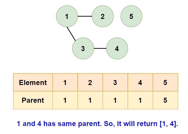
- Input: [[1,2], [1,3], [3,4], [1,4], [1,5]]

Expected Output: [1,4]
Justification: The edge [1,4] is redundant because removing it will eliminate the cycle 1-3-4-1 while keeping the graph connected.

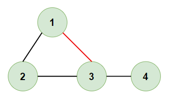
Example 2:
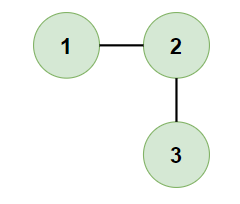
- Input: [[1,2], [2,3], [3,1], [3,4]]

Expected Output: [3,1]
Justification: The edge [3,1] creates a cycle 1-2-3-1. Removing it leaves a tree with no cycles.

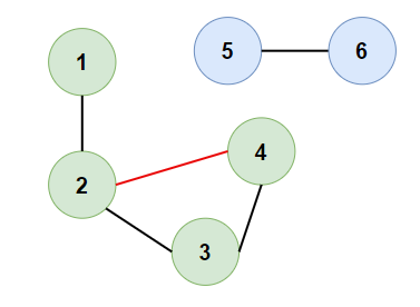
Example 3:
- Input: [[1,2], [2,3], [3,4], [4,2], [5,6]]

Expected Output: [4,2]
Justification: The edge [4,2] adds a cycle 2-3-4-2 in one part of the graph. Removing this edge breaks the cycle, and the remaining graph is a tree.

Constraints:

n == edges.length
3 <= n <= 1000
edges[i].length == 2
1 <= ai < bi <= edges.length
ai != bi
There are no repeated edges.
The given graph is connected.

Solution

The solution to this problem employs the Union-Find algorithm, which is effective for cycle detection in graphs. Initially, each node is considered as a separate set. As we iterate through the edges of the graph, we use the Union-Find approach to determine if the nodes connected by the current edge are already part of the same set. If they are, it indicates the presence of a cycle, and this edge is the redundant one. Otherwise, unite these two sets, meaning connect the nodes without forming a cycle. This approach focuses on progressively merging nodes into larger sets while keeping an eye out for the edge that connects nodes already in the same set.

Here’s how we’ll apply it:

Initialize an array to represent each node’s parent. Initially, each node is its own parent, indicating that they are each in their own separate sets.
Iterate through the list of edges. For each edge, apply the “Find” operation to both nodes. If the nodes have different parents, they belong to different sets, and we can union them by pointing the parent of one to the other.
If the “Find” operation reveals that the two nodes already share a parent, then they’re in the same set, meaning the edge under consideration creates a cycle. This edge is the redundant connection we’re looking for.
The process ends once we find the redundant connection or after processing all edges.

This approach works as it precisely detects cycles in the way trees should not have them. It’s efficient because the “Union” and “Find” operations can be optimized to almost constant time complexity with path compression and union by rank.

Algorithm Walkthrough:

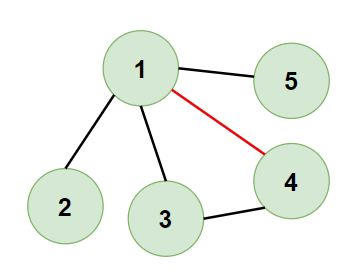
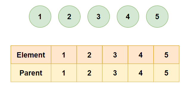
Consider the input [[1,2], [1,3], [3,4], [1,4], [1,5]].

Initialize the parent array where parent[i] = i.

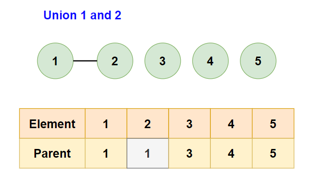
Consider the edge [1,2]:
- Find the parents of 1 and 2. Since they’re different, union them by making one the parent of the other.

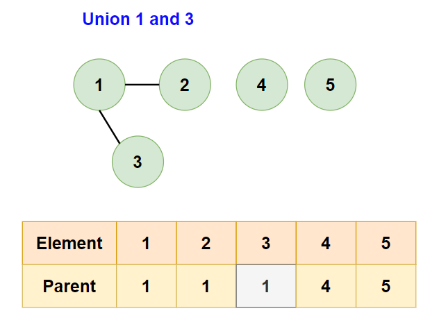
Next, consider the edge [1,3]:
- Their parents are different, so union them.

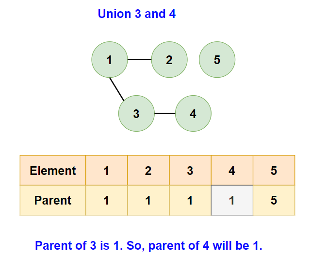
Now, consider the edge [3,4]:
- Again, different parents, so union them.

Consider the edge [1,4]:
- Find operations for both nodes return the same parent, indicating a cycle. We identify [1,4] as the redundant edge.

Code

class Solution:
    def findRedundantConnection(self, edges):
        parent = [i for i in range(len(edges) + 1)]

        def find(node):
            if parent[node] != node:
                parent[node] = find(parent[node])  # Path compression
            return parent[node]

        def union(node1, node2):
            parent[find(node1)] = find(node2)  # Union

        for edge in edges:
            node1, node2 = edge
            if find(node1) == find(node2):
                return edge  # Redundant connection found
            union(node1, node2)

        return []

if __name__ == '__main__':
    solution = Solution()

    # Test the algorithm with the three example inputs
    example1 = [[1,2], [1,3], [3,4], [1,4], [1,5]]
    example2 = [[1,2], [2,3], [3,1], [3,4]]
    example3 = [[1,2], [2,3], [3,4], [4,2], [5,6]]

    print("Example 1:", solution.findRedundantConnection(example1))
    print("Example 2:", solution.findRedundantConnection(example2))
    print("Example 3:", solution.findRedundantConnection(example3))

Complexity Analysis:

Time Complexity: The time complexity is O(N log N), where N is the number of nodes, due to the Union-Find operations with path compression over all edges.).
Space Complexity: The space complexity is (O(N)), since we maintain a parent array of size (N) where (N) is the number of vertices.

Number of Provinces

547. Number of Provinces Design Gurus

和Pattern Island中的Number of Islands 类似。这道题的matrix表示的是邻接矩阵，可以使用并查集。

同时这道题在Pattern Graph中也出现了，也可以使用DFS。

Number of Islands表示的是陆地和海洋，适合使用DFS.

Problem Statement

There are n cities. Some of them are connected in a network. If City A is directly connected to City B, and City B is directly connected to City C, city A is directly connected to City C.

If a group of cities are connected directly or indirectly, they form a province.

You are given a square matrix of size n x n, where each cell’s value indicates whether a direct connection between cities exists (1 for connected and 0 for not connected).

Determine the total number of provinces.

Examples

Example 1:
- Input: [[1,1,0],[1,1,1],[0,1,1]]

Expected Output: 1
Justification: Here, all cities are connected either directly or indirectly, forming one province.
Example 2:
- Input: [[1,0,0],[0,1,0],[0,0,1]]

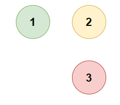
Expected Output: 3
Justification: In this scenario, no cities are connected to each other, so each city forms its own province.
Example 3:
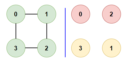
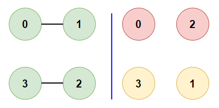
- Input: [[1,0,0,1],[0,1,1,0],[0,1,1,0],[1,0,0,1]]

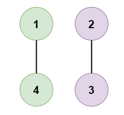
Expected Output: 2
Justification: Cities 1 and 4 form a province, and cities 2 and 3 form another province, resulting in a total of 2 provinces.

Constraints:

1 <= n <= 200
n == isConnected.length
n == isConnected[i].length
isConnected[i][j] is 1 or 0.
isConnected[i][i] == 1
isConnected[i][j] == isConnected[j][i]

Solution

To solve this problem, we’ll employ the Union-Find algorithm, a powerful tool for managing disjoint sets. The essence of the approach is to group cities into sets, where each set represents a connected province.

Initially, every city is considered its own province. As we go through the matrix, we use Union operations to join cities that are directly connected, effectively merging their sets. The Find operation identifies the representative of each set (or province) and helps in determining if two cities are already in the same province. By iteratively applying Union operations to all connected city pairs, we merge their respective sets.

In the end, the number of distinct sets (or provinces) is determined by counting the unique representatives of each set, providing the solution to our problem. This approach ensures efficient handling of connections and an accurate count of disconnected provinces.

Here’s a detailed explanation:

Initialization: We initialize an array parent to keep track of the root of each node. Each node is initially its own parent.
Union Operation: If two nodes belong to different sets (different parents), we connect them by making the root of one the parent of the other, effectively merging the sets.
Find Operation with Path Compression: When we wish to determine which set a node belongs to, we find its root. If during this search we traverse nodes, we directly connect them to the root to flatten the structure, which speeds up future ‘find’ operations.
Counting Provinces: We start with the assumption that each node is its own province. As we connect nodes, we decrement the count of provinces.

This approach is efficient due to path compression, which flattens the tree structure used internally, leading to very fast subsequent find operations.

Algorithm Walkthrough

Given an input isConnected = [[1,1,0],[1,1,0],[0,0,1]], let’s walk through the algorithm:

Initialize parent to [0, 1, 2].

Compare node 0 with node 1, they are connected. Union them, parent becomes [0, 0, 2]. Provinces decrement to 2.

Compare node 0 with node 2, no connection. Skip.
Compare node 1 with node 2, no connection. Skip.
The final count of provinces is 2.

Code

class Solution:
    def __init__(self):
        self.parent = []  # Initialize an empty list to store parent nodes.

    def find(self, i):
        if self.parent[i] != i:
            self.parent[i] = self.find(self.parent[i])  # Apply path compression to optimize the find operation.
        return self.parent[i]

    def union(self, i, j):
        self.parent[self.find(i)] = self.find(j)  # Union two nodes by updating their parent pointers.

    def findProvinces(self, isConnected):
        n = len(isConnected)
        self.parent = list(range(n))  # Initialize parent array to represent individual provinces.
        provinces = n  # Initialize the count of provinces to the total number of nodes.

        for i in range(n):
            for j in range(i + 1, n):
                if isConnected[i][j] == 1 and self.find(i) != self.find(j):
                    self.union(i, j)  # Connect nodes if they are connected and belong to different provinces.
                    provinces -= 1  # Decrement the count of provinces when merging.

        return provinces  # Return the count of provinces remaining.

# Example Test Cases
if __name__ == '__main__':
    solution = Solution()
    
    # Example 1
    example1 = [[1,1,0],[1,1,0],[0,0,1]]
    print(solution.findProvinces(example1))  # Expected Output: 2

    # Example 2
    example2 = [[1,0,0],[0,1,0],[0,0,1]]
    print(solution.findProvinces(example2))  # Expected Output: 3

    # Example 3
    example3 = [[1,0,0,1],[0,1,1,0],[0,1,1,0],[1,0,0,1]]
    print(solution.findProvinces(example3))  # Expected Output: 2

Complexity Analysis

Time Complexity: The time complexity is O(n^3) in the worst case, where n is the number of nodes. This is because the union and find operations can take O(n) time without optimizations and we perform up to O(n^2) comparisons.

However, with path compression and union by rank, the amortized time complexity of each union-find operation can be reduced to nearly O(1), making the algorithm run in nearly O(n^2) time.

Space complexity: The space complexity is O(n) for storing the parent array.

Is Graph Bipartite?

785. Is Graph Bipartite? Design Gurus

Problem Statement

Given a 2D array graph[][], representing the undirected graph, where graph[u] is an array of nodes that are connected with node u.

Determine whether a given undirected graph is a bipartite graph.

The graph is a bipartite graph, if we can split the set of nodes into two distinct subsets such that no two nodes within the same subset are adjacent (i.e., no edge exists between any two nodes within a single subset).

Examples

Example 1:
- Input: [[1,3], [0,2], [1,3], [0,2]]

Expected Output: true
Justification: The nodes can be divided into two groups: {0, 2} and {1, 3}. No two nodes within each group are adjacent, thus the graph is bipartite.

Example 2:
- Input: [[1], [0], [3], [2]]

Expected Output: true
Justification: The graph is a simple chain of 4 nodes. It’s clearly bipartite as we can have {0, 2} and {1, 3} as the two subsets.

Example 3:
- Input: [[1,2,3],[0,2],[0,1,3],[0,2]]

Expected Output: false
Justification: We found that edges (1, 2), (1, 3), and (2, 3) connect nodes within the same set, which violates the condition for a bipartite graph where each edge must connect nodes in different subsets. Thus, there’s no way to divide this graph into two subsets that satisfy the bipartite condition.

Constraints:

graph.length == n
1 <= n <= 100
0 <= graph[u].length < n
0 <= graph[u][i] <= n - 1
graph[u] does not contain u.
All the values of graph[u] are unique.
If graph[u] contains v, then graph[v] contains u.

Solution

To check if a graph can be bipartitioned, we employ the Union Find strategy. Initially, each node is treated as a distinct set, signifying that every node is in its own group. As we progress, each edge in the graph is examined. The pivotal aspect here is to determine whether the nodes connected by an edge are in different sets. If they are in the same set, it indicates a violation of the bipartition condition. For edges connecting nodes in separate sets, we perform a union operation, merging these sets. This step is crucial as it helps in grouping the nodes in a manner that allows for a potential bipartition.

Throughout this process, path compression flattens the structure of the sets, speeding up subsequent operations. The graph can be considered bipartite if, after evaluating all edges, no adjacent nodes are found in the same set. However, if any adjacent nodes are in the same set, the graph fails the bipartition test. This method effectively uses the concept of disjoint sets to determine if a given graph can be split into two groups without any overlapping edges.

Step-by-step algorithm

要看能不能分为两个部分，并且每一个部分中的任何两个节点都有相连，那就是说如果我们遍历和一个节点i相邻的所有节点的时候，这些和节点i相邻的节点应该划分为同一个簇，因为他们都不能和节点i在以一个group里，所以只能在i的对立。在遍历的过程中如果发现一个edge连接的两个点已经在一个group了，那就应该return false.

Code

class Solution:
    def isBipartite(self, graph):
        # Initialize parent list, initially each node is its own parent
        parent = [i for i in range(len(graph))]

        # Define a function to find the parent of a node using path compression
        def find(node):
            if parent[node] != node:
                parent[node] = find(parent[node])  # Path compression
            return parent[node]

        # Define a function to perform union of two nodes by updating their parents
        def union(node1, node2):
            parent[find(node1)] = find(node2)

        # Iterate through each node in the graph
        for u in range(len(graph)):
            if graph[u]:
                parentU = find(u)  # Find the parent of the current node
                firstNeighbor = graph[u][0]  # Get the first neighbor of the current node

                # Iterate through neighbors of the current node
                for v in graph[u]:
                    if find(v) == parentU:  # Check for a conflict in the same partition
                        return False  # If conflict is detected, the graph is not bipartite
                    union(firstNeighbor, v)  # Union the first neighbor with the current neighbor
        return True


# Example usage
sol = Solution()
print(sol.isBipartite([[1, 3], [0, 2], [1, 3], [0, 2]]))  # True
print(sol.isBipartite([[1], [0], [3], [2]]))  # True
print(sol.isBipartite([[1, 2, 3], [0, 2], [0, 1, 3], [0, 2]]))  # False

Complexity Analysis

Time complexity:

Each union and find operation can be considered almost O(1) due to path compression.
The main loop processes each edge once, and there are E edges in the graph.
Hence, the time complexity is O(E), where E is the number of edges in the graph.

Space complexity:

We use an array to represent the union-find structure. This array has a size equal to the number of vertices V.
Hence, the space complexity is O(V), where V is the number of vertices in the graph.

# Path With Minimum Effort

Problem Statement

Given a 2D array heights[][] of size n x m, where heights[n][m] represents the height of the cell (n, m).

Find a path from the top-left corner to the bottom-right corner that minimizes the effort required to travel between consecutive points, where effort is defined as the maximum absolute difference in height between two points in a path. In a single step, you can either move up, down, left or right.

Determine the minimum effort required for any path from the first point to the last.(找一条路径中最大的effort,并且这个effort需要是所有路径中最大effort中最小的)

Example Generation

Example 1:

Input: [[1,2,3],[3,8,4],[5,3,5]]
Expected Output: 1
Justification: The path with the minimum effort is along the edges of the grid (right, right, down, down) which requires an effort of 1 between each pair of points.

Example 2:

Input: [[1,2,2],[3,3,3],[5,3,1]]
Expected Output: 2
Justification: The path that minimizes the maximum effort goes through (1,2,2,3,1), which has a maximum effort of 2 (from 3 to 1).

Example 3:

Input: [[1,1,1],[1,1,1],[1,1,1]]
Expected Output: 0
Justification: The path that minimizes the maximum effort goes through (1,1,1,1,1), which has a maximum effort of 0.

Constraints:

rows == heights.length
columns == heights[i].length
1 <= rows, columns <= 100
1 <= heights[i][j] <= 106

Solution

To solve this problem, we’ll employ the Union Find algorithm. The core idea here is to sort all the edges (the differences in elevation between adjacent cells) in ascending order. Then, starting from the smallest edge, we’ll progressively unite adjacent cells in the grid. The process of uniting cells involves linking together cells that can be reached with the current maximum effort level. This step is crucial because it helps to build a path incrementally while ensuring that we keep the effort as low as possible.

We continue this process of uniting cells until the top-left cell and the bottom-right cell are connected. At this point, the current maximum effort level represents the minimum effort needed to traverse from the start to the end. This method efficiently finds the path with the least resistance while considering all possible paths and their associated efforts.

The algorithm involves the following steps:

Step 1: Initialization

Create a UnionFind instance for a 3x3 grid, resulting in 9 elements (0 to 8).
Initialize an empty list to store edges.

Step 2: Building Edges

Iterate over each cell in the grid.
For each cell, calculate the absolute difference in elevation with its right and bottom neighbors (if they exist).

Step 3: Sorting Edges

Sort the edges by their elevation difference in ascending order.

Step 4: Perform Union-Find Operations

For each edge in the sorted list, perform the following:
- Extract the two cells (cell1 and cell2) and their elevation difference from the edge.
- Perform the union operation on cell1 and cell2.

Step 5: Union Operation

In the union function, find the roots of both cell1 and cell2 using the find method.
If the roots are different, join the two sets. If one set has a higher rank (depth), make it the parent of the other.
If both sets have equal rank, make one the parent of the other and increase the rank of the parent.

Step 6: Find Operation

In the find method, for a given cell, find the root of the set to which it belongs.
Implement path compression: Set each cell along the way to point directly to the root. This optimizes future find operations.

Step 7: Check for Connection

After each union operation, check if the start cell (0,0) and the end cell (2,2) are connected.
This is done by checking if the roots of cell 0 and cell 8 (in the UnionFind structure) are the same.
If they are connected, stop the process.

Step 8: Result

The elevation difference of the last processed edge that connected the start and end cells is the minimum effort required.

Algorithm Walkthrough

Step 1: Initialization

Initialize a UnionFind instance for a 3x3 grid, resulting in 9 elements.
Create an empty list to store the edges.

Step 2: Building Edges

Iterate through each cell in the grid and calculate the absolute differences with its right and bottom neighbors (if they exist).
For the input [[1,2,3],[3,8,4],[5,3,5]], create edges with their differences:
- Between (0,0) and (0,1): |1-2| = 1
- Between (0,1) and (0,2): |2-3| = 1
- Between (0,0) and (1,0): |1-3| = 2
- Between (1,0) and (2,0): |3-5| = 2
- Between (1,0) and (1,1): |3-8| = 5
- Between (1,1) and (1,2): |8-4| = 4
- Between (0,1) and (1,1): |2-8| = 6
- Between (1,1) and (2,1): |8-3| = 5
- Between (0,2) and (1,2): |3-4| = 1
- Between (1,2) and (2,2): |4-5| = 1
- Between (2,0) and (2,1): |5-3| = 2
- Between (2,1) and (2,2): |3-5| = 2

Step 3: Union-Find Operations

First, we sort the edges by their differences:

Edges with Difference = 1:
- (0,0) and (0,1): Difference = 1
- (0,1) and (0,2): Difference = 1
- (0,2) and (1,2): Difference = 1
- (1,2) and (2,2): Difference = 1
Edges with Difference = 2:
- (0,0) and (1,0): Difference = 2
- (1,0) and (2,0): Difference = 2
- (2,0) and (2,1): Difference = 2
- (2,1) and (2,2): Difference = 2
Edges with Higher Differences (not initially relevant for the desired path).

Now, let’s perform the Union-Find operations:

Processing Edges with Difference = 1

Union (0,0) and (0,1):
- Connects cells 0 and 1. Parents: [0, 0, 2, 3, 4, 5, 6, 7, 8].
Union (0,1) and (0,2):
- Connects cells 1 and 2 (and hence 0 with 2). Parents: [0, 0, 0, 3, 4, 5, 6, 7, 8].
Union (0,2) and (1,2):
- Connects cells 2 and 5. Parents: [0, 0, 0, 3, 4, 0, 6, 7, 8].
Union (1,2) and (2,2):
- Connects cells 5 and 8. Parents: [0, 0, 0, 3, 4, 0, 6, 7, 0].
- At this step, cells 0 and 8 are connected.

The last edge difference is 1.

Code

class UnionFind:
    def __init__(self, size):
        self.parent = [i for i in range(size)]  # Initialize parent array
        self.rank = [0] * size  # Initialize rank array

    def find(self, x):
        if self.parent[x] != x:  # Path compression: If x is not its own parent, find its root parent.
            self.parent[x] = self.find(self.parent[x])
        return self.parent[x]

    def union(self, x, y):
        rootX = self.find(x)  # Find root parent of x
        rootY = self.find(y)  # Find root parent of y
        if rootX != rootY:  # Union the sets if they have different root parents
            if self.rank[rootX] > self.rank[rootY]:  # Union by rank: Attach the shorter tree to the taller one
                self.parent[rootY] = rootX
            elif self.rank[rootX] < self.rank[rootY]:
                self.parent[rootX] = rootY
            else:  # If ranks are equal, choose any root to be the new parent and increase rank
                self.parent[rootY] = rootX
                self.rank[rootX] += 1


class Solution:
    def minimumEffortPath(self, heights):
        row, col = len(heights), len(heights[0])
        uf = UnionFind(row * col)  # Initialize Union-Find data structure
        edges = []

        for i in range(row):
            for j in range(col):
                if i > 0:  # Add edge to the cell above (if it exists)
                    edges.append((i * col + j, (i - 1) * col + j, abs(heights[i][j] - heights[i - 1][j])))
                if j > 0:  # Add edge to the cell on the left (if it exists)
                    edges.append((i * col + j, i * col + (j - 1), abs(heights[i][j] - heights[i][j - 1])))

        edges.sort(key=lambda x: x[2])  # Sort edges by the difference in heights

        for x, y, diff in edges:  # Iterate through sorted edges
            uf.union(x, y)  # Union the cells connected by the edge
            if uf.find(0) == uf.find(
                    row * col - 1):  # If the source and destination cells are connected, return the effort
                return diff

        return 0


# Examples
sol = Solution()
print("Example 1:", sol.minimumEffortPath([[1, 2, 3], [3, 8, 4], [5, 3, 5]]))  # Expected Output: 1
print("Example 2:", sol.minimumEffortPath([[1, 2, 2], [3, 3, 3], [5, 3, 1]]))  # Expected Output: 2
print("Example 3:", sol.minimumEffortPath([[1, 1, 1], [1, 1, 1], [1, 1, 1]]))  # Expected Output: 0

Complexity Analysis

Time Complexity:

The time complexity of this algorithm is primarily dictated by the sorting of the edges.
If there are n cells, we can have at most 2n edges (since each cell can have at most 2 outgoing edges to its right and bottom neighbors).
Sorting 2n edges takes O(2n log(2n)), which simplifies to O(n log n).
The union-find operations (find and union) take O(n) time each.
Hence, the overall time complexity is O(n log n).

Space Complexity:

The space complexity is O(n) for storing the parents and ranks in the union-find data structure and the edge list.

Author：Hasuer

Link：https://hasuer.github.io/25-pattern-union-find/index.html

Publish date：May 25th 2024, 2:26:45 pm

Update date：May 28th 2024, 11:31:01 am

License：本文采用知识共享署名-非商业性使用 4.0 国际许可协议进行许可

Next Post

26. Pattern Ordered Set
Previous Post

24. Pattern Topological Sort (Graph)

CATALOG

1. Introduction to Union Find Pattern
2. Redundant Connection
3. Number of Provinces
4. Is Graph Bipartite?
5. # Path With Minimum Effort