
Introduction to Hashing
Imagine you have a huge bookshelf (like, Hogwarts library size). You’ve got a new book and need to find a spot for it and later on, search it quickly every time you need it. Instead of scanning the whole shelf, you use a magical spell that tells you exactly where to place or find it. This magical spell takes the book’s title and gives you a specific location, like “4th shelf, 10th spot”. But remember! Even if you slightly change the book’s title, the spell gives a completely different spot.
Now, let’s map this to computer science:
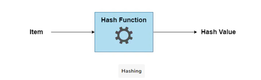
Hashing: It’s a technique that takes an input (or ‘message’) and returns a fixed-size string, which looks random. The output, known as the hash value, is unique (mostly) to the given input.
Hash Function: This is our “magical spell” that converts the input data (like our book title) into a fixed-length value.
However, no magic is perfect. If two different inputs give the same hash, that’s called a collision. It’s like our spell accidentally pointing to the same spot for two different books. Good hash functions make these super rare. We will discuss this in detail later on.
The following illustration depicts a generalized hashing scenario.
But why hashing is important? Let’s find out!
Why hashing?
Hashing is a great tool to quickly access, protect, and verify data. Here are a few of the common use cases of hashing:
- Quick Data Retrieval: Hashing helps in accessing data super fast. With it, systems can quickly find a data piece without searching the whole database or list.
- Data Integrity Checks: When downloading a file from the web, the site may provide you with a hash value for that file. If even a tiny portion of that file changes during the download, its hash will differ. By comparing the provided hash with the hash of the downloaded file, you can determine whether the file is exactly as the original, or if it was tampered with during the transfer
- Password Security: Instead of storing actual passwords, systems store their hash. It’s like locking the real magical item away and just keeping a hologram on display.
- Hash Tables: Hashing is used in programming for efficient data structures like hash tables. It’s like having organized shelves for our books where each item has its designated spot.
- Cryptography: Some hash functions are used in cryptography to ensure data confidentiality and integrity. It’s like a spell that only allows certain wizards to read a message.
- Data Deduplication: If you’re saving data, and you don’t want duplicates, you can just compare their hashes. Same hash? It’s the same data. It ensures you’re not wasting space with repeated magical items.
- Load Balancing: In big systems serving many users, hashes can be used to decide which server should handle a particular request. It’s like deciding which magical portal to send a wizard based on their wand.
Hashing has numerous applications in several practical domains. However, this section tries to cover Hashing for defining and implementing a retrieval efficient data structure called Hash Table, which will be our next lesson.
Introduction to Hash Tables
A Hash Table (also known as Hash Map), at its core, is a data structure that allows us to store and retrieve data efficiently. If we think about a real-life analogy, it’s like a library where each book (data) has a unique identifier (key) like ISBN, and all books are organized in a specific way to allow the librarian (hash function) to find and retrieve them quickly.
In other words, a Hash Table implements an associative array abstract data type (or Dictionary ADT), mapping keys to values. A Hash Table uses a hash function to compute an index into an array of buckets or slots where the desired value is stored.
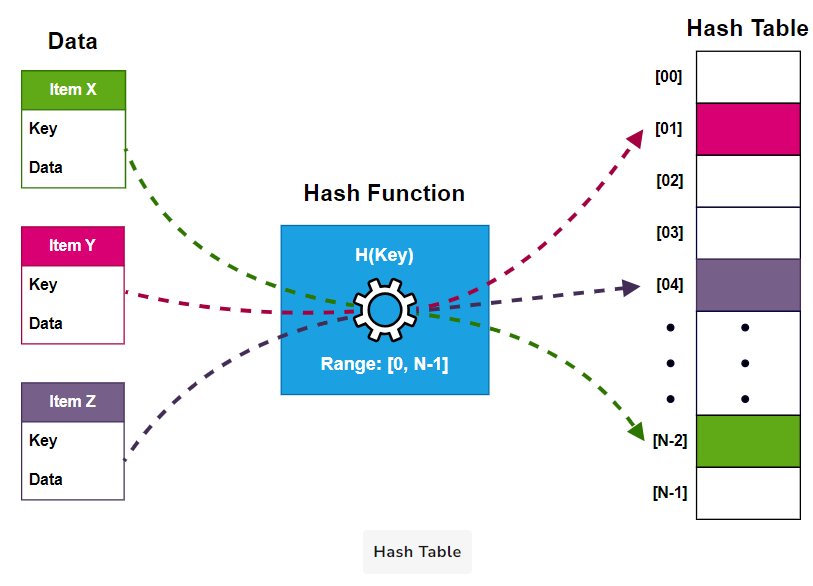
There are four main elements to any Hash Table: Keys, Values, the Hash Function, and Buckets.
- Keys: In our library analogy, think of keys as the unique identifiers for each book. Keys are the inputs we feed into our hash function. They can be any data type - numbers, strings, or even objects. The crucial characteristic of keys is that they should be unique. If two pieces of data share the same key, it might lead to complications, like collisions (we’ll discuss this in detail later).
- Values: Values are the actual data that we store in our Hash Table. They could be anything from a single number to a complex object or even a function. Using the key, we can quickly retrieve the corresponding value from the Hash Table.
- Hash Function - H(x): We’ve touched on this before, but it’s worth emphasizing the importance of the hash function. This is the engine that drives a Hash Table. It’s responsible for transforming keys into hash values, which dictate where we store our data in the table.
- Buckets: Once the hash function processes our key, it produces a hash value. This value corresponds to a specific location or ‘bucket’ within the Hash Table. Think of buckets as shelves in our library, each one designated to store a specific book (or piece of data).
Here are the three basic operations that are performed on Hash Tables:
- Insert(key, value) operation: Calculates the hash index H(key) and stores the key-value pair in the slot at that index.
- Search(key) operation: Computes H(key) to find the slot and returns the value associated with the key, or
nullif not present. - Delete(key) operation: Removes the key-value pair stored at index H(key).
A naive Hash Table implementation
Imagine once again a major public library that needs to store basic information, such as Key (ISBN), Title, and Placement Info, for all available books. This system is heavily used, with librarians frequently searching for books. This results in many retrieval requests.
The frequent retrievals require an efficient solution that can quickly perform the search operation (ideally, in constant time). Therefore, the Hash table data structure perfectly suits the scenario.
Let’s start by discussing our data model. We will use a dynamic array of the Record type to store the books’ information. Here is what our Record class looks like:
1 | class Record: |
ADT class
Now, let’s look at the HashTable ADT class definition. The HashTable class has an HT_array pointer to store the address of the dynamically allocated array of records. The max_length property is the maximum number of records the hash table can hold. The length represents the current number of records in the Hash table. It increments and decrements with insertions and deletions, respectively.
1 | class HashTable: |
Defining the hash method
Let’s define our Hash method H() for this naive implementation. We will use the simplest modular Hashing for this scenario:
1 | def H(self, key): |
The above Hash function ensures we always get an index value in the range [0, max_length - 1]. Let’s move on to see how the simplified/ naive Insert() method works.
Naive insertion operation
The Insert() method takes a new record as a parameter and checks if the maximum capacity of the HT_array is not reached. If the table still can have more records, the method calculates a proper index/ hash key for placing this item. After that, it puts the item at the computed index.
1 | def Insert(self, item): |
Point to ponder: What happens if two different keys map to the same array index? This implementation overwrites it. Indeed, it is a flaw we will address in the Solving Collisions section.
Naive search operation
Now, let’s explore how and why the Search() method will retrieve records in O(1) for us. Here is a naive implementation:
1 | def Search(self, key, returnedItem): |
The Search() method applies the hash function H() on the passed key and checks if the hash table slot is empty or not. If this slot has a valid record, the Search() method assigns the record at this slot to the reference parameter. Also, it returns a true flag to indicate the operation’s success.
The above implementation of Search() clearly takes constant time (i.e., ) time to retrieve/ search any record regardless of the size our table may grow. This is evident by the fact that you only have to apply the hash function only constant number of times to calculate the position of the searched item.
Note: This naive implementation for the search doesn’t cover all aspects. We will discuss a more sophisticated method in the next lesson.
Naive delete operation
Like the search operation, this deletion operation first locates the item requiring a delete. Afterward, the deletion operation simply places a null or default object at the table slot.
Here is what the naive implementation looks like:
1 | def Delete(self, key): |
Again, like the search operation, deletion also takes a constant time to locate and delete an item from the table. But, it is important to note that this naive implementation is just to get an overall idea of how the hash table works. However, it doesn’t cater to many exceptional cases; we will discuss those in the subsequent sections.
Here is the complete code for the naive hash table implementation with a sample driver code:
1 | class Record: |
Implementation
Here is how different languages have implemented Hash Tables:
| Language | API |
|---|---|
| Java | java.util.Map Or java.util.HashMap |
| Python | dict |
| C++ | std::unordered_map |
| JavaScript | Object or Map |
Issues with Hash Tables
Remember, we said that our earlier Hash Table implementation was naive. By that, we meant that the code doesn’t cater to some frequently occurring issues. Let’s see what these issues really are.
Collisions
A collision in a Hash Table occurs when an insert operation tries to insert an item at a table slot already occupied by another item. How can this ever happen? Let’s find out.
Collision example
Reconsider our earlier example of the Hash Table for the public library book information storage. Assume, for the sake of simplicity, the Hash Table has the max_length equal to 10. Further, you need to insert the following book records in it:
| Key | Title | Placement Info |
|---|---|---|
| 1008 | Introduction to Algorithms | A1 Shelf |
| 1009 | Data Structures: A Pseudocode Approach | B2 Shelf |
| 1010 | System Design Interview Roadmap | C3 Shelf |
| 1011 | Grokking the Coding Interview | D4 Shelf |
| 1021 | Grokking the Art of Recursion for Coding Interviews | E5 Shelf |
Here is the hash value calculation for the first four entries:
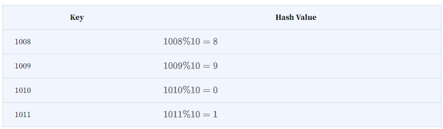
So the hash table array would look something like this:
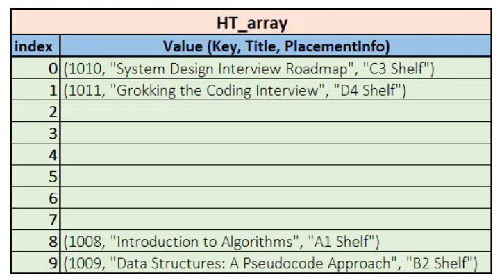
Now, what happens if we try inserting the record with the Key 1021? The hash value for 1021 is the same as occupied by the book with the Key 1011. In this scenario, we say that a collision has occurred.
The phenomenon is depicted in the following illustration.

Collisions occur frequently in hash tables when two different keys hash to the same bucket. Without proper collision handling, lookup performance degrades from O(1) to O(n) linear search time. Managing collisions is crucial to efficient hash table implementation.
Overflows
Overflow in a hash table occurs when the number of elements inserted exceeds the fixed capacity allocated for the underlying bucket array. For example, if you already have inserted information of ten books in the earlier discussed hash table, inserting the 11th one will cause an overflow.
One important point to note here is that as the underlying bucket array starts filling towards its maximum capacity, the expectation of collisions starts increasing. Thereby the overall efficiency of hash table operations starts decreasing.
An ideal hash table implementation must resolve collisions effectively and must act to avoid any overflow early. In the next section, we will explore different strategies for handling collisions.
Resolving Collisions
Remember that our naive hash table implementation directly overwrote existing records when collisions occurred. This is inaccurate as it loses data on insertion. This section describes how we can avoid such data losses with the help of collision resolution techniques.
Based on how we resolve the collisions, the collision resolution techniques are classified into two types:
- Open addressing / Closed hashing
- Chaining / Open hashing
Let’s find out how these schemes help us resolve the collisions without losing any data.
Open Addressing (Closed Hashing):
Open addressing techniques resolve hash collisions by probing for the next available slot within the hash table itself. This approach is called open addressing since it opens up the entire hash table for finding an empty slot during insertion.
It is also known as closed hashing because the insertion is restricted to existing slots within the table without using any external data structures.
Depending on how you jump or probe to find the next empty slot, the closed hashing is further divided into multiple types. Here are the main collision resolution schemes used in the open-addressing scheme:
- Linear probing: Linear probing is the simplest way to handle collisions by linearly searching consecutive slots for the next empty location.
- Quadratic probing: When a collision occurs, the quadratic probing attempts to find an alternative empty slot for the key by using a
quadratic functionto probe the successive possible positions. - Double hashing: It uses two hash functions to determine the next probing location in case of a successive collision.
- Random probing: Random probing uses a pseudo-random number generator (PRNG) to compute the step size or increment value for probes in case of collisions.
Implementation of insertion, search, and deletion operations is slightly different for each type of the operations.
Separate Chaining (Open Hashing):
Selecting the right closed hashing technique for resolving collisions can be tough. You need to keep the pros and cons of different strategies in mind and then have to make a decision.
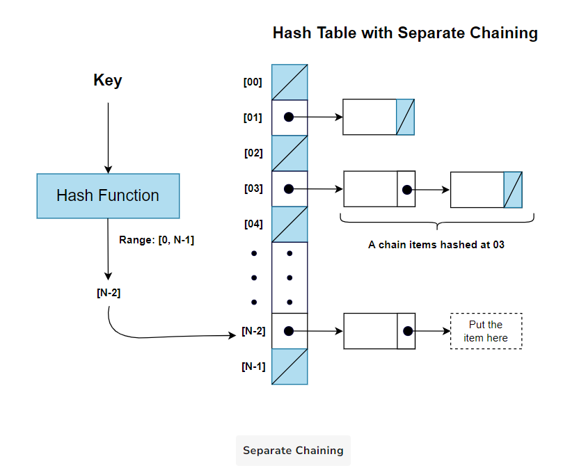
Separate chaining offers a rather simpler chaining mechanism to resolve collisions. Each slot in the hash table points to a separate data structure, such as a linked-list. This linked-list or chain stores multiple elements that share the same hash index. When a collision occurs, new elements are simply appended to the existing list in the corresponding slot.
Separate chaining is an “open hashing” technique because the hash table is “open” to accommodate multiple elements within a single bucket (usually using a chain) to handle collisions. Here is the generalized conceptual diagram for the chaining method:
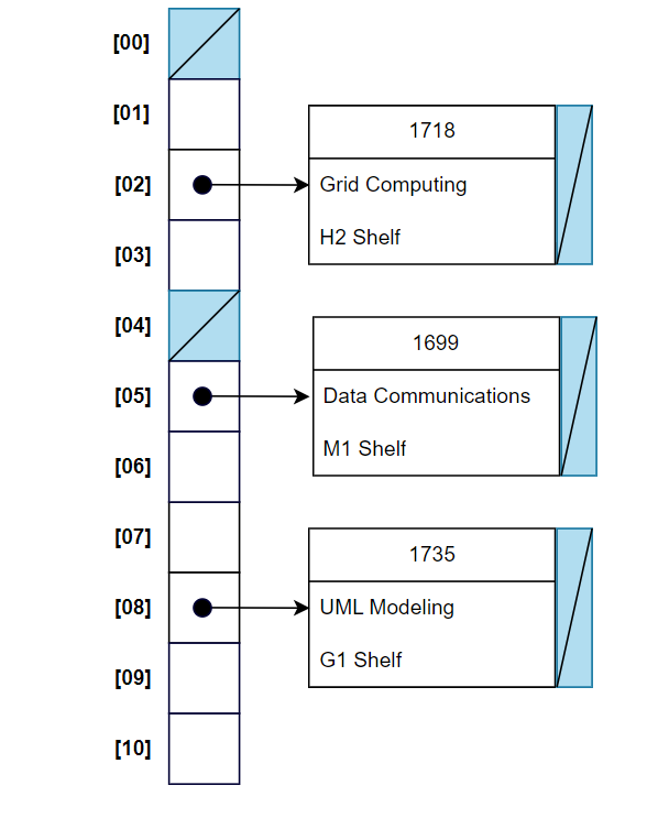
Example: Recall our earlier example of the hash table for storing books’ information. Assume you have a hash table (with open hashing) of size 11 and have the following situation:
Now, here is what the hash table would look like after inserting a new book record (1724, "Compilers Theory", "E4 Shelf"):
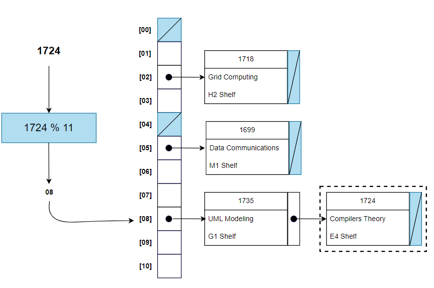
The key 1724 hashes on 08. Therefore, the item with this key is appended at the end of the chain, pointed by table slot 08.
Let’s now move on to implementing the hash table with separate chaining.
A complete implementation
Insertion in a hash table with separate chaining is simple. For an item with hash key x, you need to just append the item at the list/ chain linked to the x slot of the table. Similarly, deletion operation is also more straightforward. You don’t need to keep any deletion signs or marks. You can directly delete the item’s node from the chain linked to the relevant hash table slot.
Here is a complete implementation of the hash table we developed for books storage:
1 | class Record: |
Perks of separate chaining
Separate chaining has the following perks over the closed hashing techniques:
- Dynamic Memory Usage: Insertions append new nodes at the chains. Unlike closed hashing, where we just put deletion mark, deleting items causes their nodes to completely removed from the chain. Thereby, the table with separate chaining can grow and shrink as per number of elements.
- Simple Implementation: Implementing separate chaining is straightforward, using linked lists to manage collisions, making the code easy to understand and maintain.
- Graceful Handling of Duplicates: This technique gracefully handles duplicate keys, allowing multiple records with the same key to be stored and retrieved accurately.
Downsides of separate chaining
Separate chaining has the following downsides:
- Increased Memory Overhead: Separate chaining requires additional memory to store pointers or references to linked lists for each bucket, leading to increased memory overhead, especially when dealing with small data sets.
- Cache Inefficiency: As separate chaining involves linked lists, cache performance can be negatively impacted due to non-contiguous memory access when traversing the lists, reducing overall efficiency.
- External Fragmentation: The dynamic allocation of memory for linked lists can lead to external fragmentation, which may affect the performance of memory management in the system.
- Worst-Case Time Complexity: In the worst-case scenario, when multiple keys are hashed to the same bucket and form long linked lists, the time complexity for search, insert, and delete operations can degrade to O(n), making it less suitable for time-critical applications.
- Memory Allocation Overhead: Dynamic memory allocation for each new element can add overhead and might lead to performance issues when the system is under high memory pressure.
Handling Overflows
Closed hashing techniques like linear probing experience overflow when entries fill up the fixed hash table slots. Overflow can loosely indicate that the table has exceeded the suitable load factor.
Ideally, for closed hashing, the load-factor a = n / m should not cross 0.5, where n is the number of entries and m is table size. Otherwise, the hash table experiences a significant increase in collisions, problems in searching, and degrading performance and integrity of the table operations.
Chaining encounters overflow when chain lengths become too long, thereby increasing the search time. The load-factor a can go up to 0.8 or 0.9 before performance is affected.
Resizing the hash table can help alleviate the overflow issues. Let’s explore what resizing is and when it is suitable to do.
Resizing
Resizing is increasing the size of the hash table to avoid overflows and maintain certain load-factor. Once the load-factor of the hash table increases a certain threshold (e.g., 0.5 for closed hashing and 0.9 for chaining), resizing gets activated to increase the size of the table.
When resizing, do the old values remain in the same place in the new table? The answer is “No.” As resizing changes the table size, the values must be rehashed to maintain the correctness of the data structure.
Rehashing
Rehashing involves applying a new hash function (s) to all the entries in a hash table to make the table more evenly distributed. In context to resizing, it means recalculating hashes (according to the new table size) of all the entries in the old table and re-inserting those in the new table. Rehashing takes O(n) time for n entries.
After rehashing, the new distribution of entries across the larger table leads to fewer collisions and improved performance. We perform rehashing periodically when the load-factor exceeds thresholds or based on metrics like average chain length.
Resizing and Rehashing Process:
- Determine that the load-factor has exceeded the threshold (e.g., alpha > 0.5 ) and that the hash table needs resizing.
- Create a new hash table with a larger capacity (e.g., double the size of the original table).
- Iterate through the existing hash table and rehash each element into the new one using the primary hash function with the new table size.
- After rehashing all the elements, the new hash table replaces the old one, and the old table is deallocated from memory.
Selecting a Hash Function
Throughout the hashing portion, we discussed only one or two hash functions. The question arises, how to develop a new hash function? Is there any technique to make your customized hash function? Let’s find out the answers.
But first, we must know how to distinguish between a good and a bad hash function. Here are some ways to explain the characteristics of a good hash function in simple terms:
Characteristics of a good hash function:
Here are some characteristics that every good hash function must follow: -
- Uniformity and Distribution: The hash function should spread out keys evenly across all slots in the hash table. It should not cram keys into only a few slots. Each slot should have an equal chance of being hashed to, like spreading items randomly across shelves. This ensures a balanced distribution without crowded clusters in some places.
- Efficiency: It should require minimal processing power and time to compute. Complex and slow hash functions defeat the purpose of fast lookup. The faster, the better.
- Collision Reduction: Different keys should end up getting mapped to different slots as much as possible. If multiple keys keep colliding in the same slot, the hash table operations will deteriorate time efficiency over time.
Hash function design techniques:
Here are a few of the commonly used techniques for creating good hash functions:
Division method
The division method is one of the simplest and most widely used techniques to compute a hash code. It involves calculating the remainder obtained by dividing the key by the size of the hash table (the number of buckets). The remainder is taken as the hash code. Mathematically, the division method is expressed as: hash_key = key % table_size.
The division method is simple to implement and computationally efficient. However, it may not be the best choice if the key distribution is not uniform or the table size is not a prime number, which may lead to clustering.
Folding method
The folding method involves dividing the key into smaller parts (subkeys) and then combining them to calculate the hash code. It is particularly useful when dealing with large keys or when the key does not evenly fit into the hash table size.
There are several ways to perform folding:
- Digit sum:
Split the key into groups of digits, and their sum is taken as the hash code. For example, you can hash the key 541236 using digit sum folding into a hash table of size 5 as: hash_key = (5+4+1+2+3+6)%2 = 21%5 = 1 .
- Reduction:
Split the key in folds and use a reduction using any associative operation like XOR to reduce folds to a single value. Now, pass this single value through the simple division hash function to generate the final hash value.
For example, suppose you want a 12-digit key 593048892357 to be hashed onto a table of size 11113. In folding with reduction, you will split it into 3 parts of 4 digits each: 5930,4889,2357. Then, you XOR (^) the parts and pass through an ordinary hash function as: hash_key=(5930 ^ 4889 ^ 2357)%table_size = 7041.
We can also add the parts: hash_key = (5930 + 4889 + 2357) % table_size = 13176 % 11113=2063
The folding method can handle large keys efficiently and provides better key distribution than the division method. It finds common applications where the keys are lengthy or need to be split into subkeys for other purposes.
Mid-square Method:
The mid-square method involves squaring the key, extracting the middle part, and then using it as the hash code. This technique is particularly useful when keys are short and do not have patterns in the lower or upper digits. The steps for calculating mid-square are as follows:
- Square the key.
- Extract the K middle digits of the square.
- Apply simple division on these middle digits to get the final hash.
For example, consider the key 3729, and we want to hash it into a hash table of size 10.
- Square the key: 3729x3729=13935241.
- Extract the middle digits to get the hash value: 935.
- Calculate the hash index: H(3729)=935%10=5.
Therefore, the key 3729 is hashed into the hash table at index 5.
The mid-square method is easy to implement and works well when the key values are uniformly distributed, providing a good spread of hash codes. However, it may not be suitable for all types of keys, especially those with patterns or significant leading/trailing zeros.
In the next section, we will solve some coding interview problems related to Hash Tables.
First Non-repeating Character (easy)
387. First Unique Character in a String Design Gurus
Problem Statement
Given a string, identify the position of the first character that appears only once in the string. If no such character exists, return -1.
Examples
- Example 1:
- Input: “apple”
- Expected Output: 0
- Justification: The first character ‘a’ appears only once in the string and is the first character.
- Example 2:
- Input: “abcab”
- Expected Output: 2
- Justification: The first character that appears only once is ‘c’ and its position is 2.
- Example 3:
- Input: “abab”
- Expected Output: -1
- Justification: There is no character in the string that appears only once.
Constraints:
- 1 <= s.length <= 10^5
sconsists of only lowercase English letters.
Solution
To solve this problem, we’ll use a hashmap to keep a record of each character in the string and the number of times it appears. First, iterate through the string and populate the hashmap with each character as the key and its frequency as the value. Then, go through the string again, this time checking each character against the hashmap. The first character that has a frequency of one (indicating it doesn’t repeat) is your target. This character is the first non-repeating character in the string. If no such character exists, the solution should indicate that as well. This two-pass approach ensures efficiency, as each character is checked against a pre-compiled frequency map.
- Initialization: Begin by creating a hashmap to store the frequency of each character in the string. This hashmap will help in identifying characters that appear only once.
- Frequency Count: Traverse the string from the beginning to the end. For each character, increment its count in the hashmap.
- First Unique Character: Traverse the string again from the beginning. For each character, check its frequency in the hashmap. If the frequency is 1, return its position as it’s the first unique character.
- No Unique Character: If the string is traversed completely without finding a unique character, return -1.
Using a hashmap ensures that we can quickly determine the frequency of each character without repeatedly scanning the string.
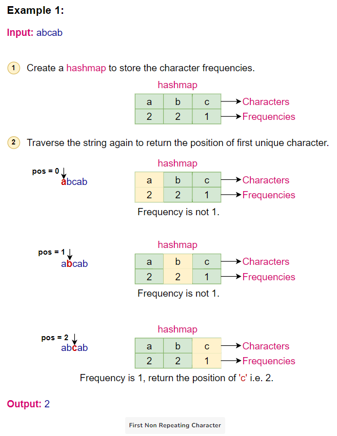
Algorithm Walkthrough:
Given the input string “abcab”:
- Initialize a hashmap to store character frequencies.
- Traverse the string:
- ‘a’ -> frequency is 1
- ‘b’ -> frequency is 1
- ‘c’ -> frequency is 1
- ‘a’ -> frequency is 2
- ‘b’ -> frequency is 2
- Traverse the string again:
- ‘a’ has frequency 2
- ‘b’ has frequency 2
- ‘c’ has frequency 1, so return its position 2.
Here is the visual representation of the algorithm:
Code
Here is the code for this algorithm:
1 | class Solution: |
Time Complexity
- Populating the hashmap with frequencies: We traverse the entire string once to populate the hashmap with the frequency of each character. This operation takes O(n) time, where n is the length of the string.
- Finding the first unique character: We traverse the string again to find the first character with a frequency of 1. This operation also takes O(n) time.
Given that these two operations are sequential and not nested, the overall time complexity is O(n) + O(n), which simplifies to O(n).
Space Complexity
- Hashmap for frequencies: In the worst case, every character in the string is unique. For a string with only lowercase English letters, the maximum number of unique characters is 26. However, if we consider all possible ASCII characters, the number is 128. If we consider extended ASCII, it’s 256. In any case, this is a constant number. Therefore, the space complexity for the hashmap is O(1) because it doesn’t grow proportionally with the size of the input string.
- Input string: The space taken by the input string is not counted towards the space complexity, as it’s considered input space.
Given the above, the overall space complexity of the algorithm is O(1).
Conclusion
The approach is efficient in terms of both time and space. The time complexity is linear, which means the algorithm’s runtime grows linearly with the size of the input. The space complexity is constant, indicating that the amount of additional space (memory) the algorithm uses does not grow with the size of the input.
Largest Unique Number (easy)
Leetcode 会员 Design Gurus
Problem Statement
Given an array of integers, identify the highest value that appears only once in the array. If no such number exists, return -1.
Examples:
- Example 1:
- Input: [5, 7, 3, 7, 5, 8]
- Expected Output: 8
- Justification: The number 8 is the highest value that appears only once in the array.
- Example 2:
- Input: [1, 2, 3, 2, 1, 4, 4]
- Expected Output: 3
- Justification: The number 3 is the highest value that appears only once in the array.
- Example 3:
- Input: [9, 9, 8, 8, 7, 7]
- Expected Output: -1
- Justification: There is no number in the array that appears only once.
Constraints:
1 <= nums.length <= 20000 <= nums[i] <= 1000
Solution
To solve this problem, we utilize a hashmap to track the frequency of each number in the given array. The key idea is to iterate through the array, recording the count of each number in the hashmap. Once all elements are accounted for, we scan through the hashmap, focusing on elements with a frequency of one. Among these, we identify the maximum value. This approach ensures that we effectively identify the largest number that appears exactly once in the array, leveraging the hashmap for efficient frequency tracking and retrieval.
- Initialization: Start by creating a hashmap that will be used to store the frequency of each number in the array. This hashmap will be instrumental in identifying numbers that appear only once.
- Frequency Count: Traverse the entire array from the beginning to the end. For each number encountered, increment its count in the hashmap. This step ensures that by the end of the traversal, we have a complete record of how many times each number appears in the array.
- Identify Largest Unique Number: After populating the hashmap, traverse it to identify numbers with a frequency of 1. While doing so, keep track of the largest such number. If no number with a frequency of 1 is found, the result will be -1.
- Return Result: The final step is to return the largest number that has a frequency of 1. If no such number exists, return -1.
This approach, which leverages the properties of a hashmap, ensures that we can quickly determine the frequency of each number without the need for nested loops or repeated scans of the array.
Algorithm Walkthrough:
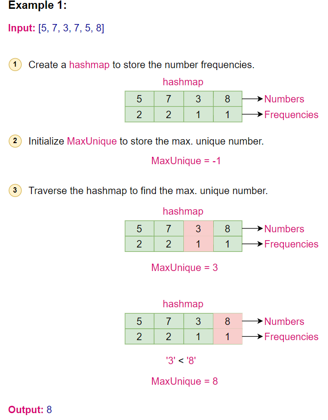
Given the input array [5, 7, 3, 7, 5, 8]:
- Initialize a hashmap to store number frequencies.
- Traverse the array:
- 5 -> frequency is 1
- 7 -> frequency is 1
- 3 -> frequency is 1
- 7 -> frequency is 2
- 5 -> frequency is 2
- 8 -> frequency is 1
- Traverse the hashmap:
- 5 has frequency 2
- 7 has frequency 2
- 3 has frequency 1
- 8 has frequency 1, and it’s the largest unique number.
Here is the visual representation of the algorithm:
Code
Here is the code for this algorithm:
1 | from collections import defaultdict |
Complexity Analysis
Time Complexity: The algorithm traverses the array once to populate the hashmap and then traverses the hashmap to find the largest unique number. Both operations are O(n), where n is the length of the array. Therefore, the overall time complexity is O(n).
Space Complexity: The space complexity is determined by the hashmap, which in the worst case will have an entry for each unique number in the array. Therefore, the space complexity is O(n), where n is the number of unique numbers in the array.
Maximum Number of Balloons (easy)
1189. Maximum Number of Balloons Design Gurus
Problem Statement
Given a string, determine the maximum number of times the word “balloon” can be formed using the characters from the string. Each character in the string can be used only once.
Examples:
- Example 1:
- Input: “balloonballoon”
- Expected Output: 2
- Justification: The word “balloon” can be formed twice from the given string.
- Example 2:
- Input: “bbaall”
- Expected Output: 0
- Justification: The word “balloon” cannot be formed from the given string as we are missing the character ‘o’ twice.
- Example 3:
- Input: “balloonballoooon”
- Expected Output: 2
- Justification: The word “balloon” can be formed twice, even though there are extra ‘o’ characters.
Constraints:
- 1 <= text.length <= 10^4
textconsists of lower case English letters only.
Solution
To solve this problem, you start by creating a hashmap to count the frequency of each letter in the given string. Since the word “balloon” contains specific letters with varying frequencies (like ‘l’ and ‘o’ appearing twice), you need to account for these in your hashmap. Once you have the frequency of each letter, the next step is to determine how many times you can form the word “balloon”. This is done by finding the minimum number of times each letter in “balloon” appears in the hashmap. The limiting factor will be the letter with the minimum frequency ratio to its requirement in the word “balloon”. This approach ensures a balance between utilizing the available letters and adhering to the letter composition of “balloon”.
- Character Frequency Count: Traverse the string and populate a hashmap with the frequency count of each character.
- Determine Maximum Count: Check the hashmap to determine the maximum number of times the word “balloon” can be formed. For characters ‘b’, ‘a’, and ‘n’, their frequency in the hashmap directly gives the number of times they can be used. For ‘l’ and ‘o’, we need to divide their frequency by 2.
- Result Calculation: The minimum value among the counts of ‘b’, ‘a’, ‘l’/2, ‘o’/2, and ‘n’ will give the maximum number of times the word “balloon” can be formed.
- Return the Result: Return the calculated minimum value as the final result.
This approach is effective because it ensures that we account for the frequency of each character required to form the word “balloon”. Using a hashmap allows for efficient storage and retrieval of character frequencies.
Algorithm Walkthrough:
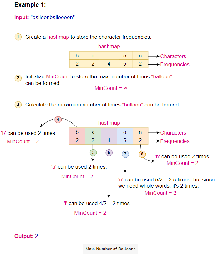
Given the input string “balloonballoooon”:
- Initialize an empty hashmap.
- Traverse the string and populate the hashmap with character frequencies: {‘b’:2, ‘a’:2, ‘l’:4, ‘o’:5, ‘n’:2}.
- Calculate the maximum number of times “balloon” can be formed:
- ‘b’ can be used 2 times.
- ‘a’ can be used 2 times.
- ‘l’ can be used 4/2 = 2 times.
- ‘o’ can be used 5/2 = 2.5 times, but since we need whole words, it’s 2 times.
- ‘n’ can be used 2 times.
- The minimum among these values is 2, which is the final result.
Here is the visual representation of the algorithm:
Code
Here is the code for this algorithm:
1 | from collections import defaultdict |
Complexity Analysis
Time Complexity: The algorithm traverses the string once to populate the hashmap, which is O(n), where n is the length of the string. The subsequent operations are constant time. Therefore, the overall time complexity is O(n).
Space Complexity: The space complexity is determined by the hashmap, which in the worst case will have an entry for each unique character in the string. However, since the English alphabet has a fixed number of characters, the space complexity is O(1).
Longest Palindrome(easy)
409. Longest Palindrome Design Gurus
Problem Statement:
Given a string, determine the length of the longest palindrome that can be constructed using the characters from the string. Return the maximum possible length of the palindromic string.
Examples:
- Input: “applepie”
- Expected Output: 5
- Justification: The longest palindrome that can be constructed from the string is “pepep”, which has a length of 5. There are are other palindromes too but they all will be of length 5.
- Input: “aabbcc”
- Expected Output: 6
- Justification: We can form the palindrome “abccba” using the characters from the string, which has a length of 6.
- Input: “bananas”
- Expected Output: 5
- Justification: The longest palindrome that can be constructed from the string is “anana”, which has a length of 5.
Constraints:
1 <= s.length <= 2000sconsists of lowercase and/or uppercase English letters only.
Solution
To solve this problem, we can use a hashmap to keep track of the frequency of each character in the string. The idea is to use pairs of characters to form the palindrome. For example, if a character appears an even number of times, we can use all of them in the palindrome. If a character appears an odd number of times, we can use all except one of them in the palindrome. Additionally, if there’s any character that appears an odd number of times, we can use one of them as the center of the palindrome.
- Initialization: Start by initializing a hashmap to keep track of the characters and their frequencies.
- Character Counting: Iterate through the string and populate the hashmap with the frequency of each character.
- Palindrome Length Calculation: For each character in the hashmap, if it appears an even number of times, add its count to the palindrome length. If it appears an odd number of times, add its count minus one to the palindrome length. Also, set a flag indicating that there’s a character available for the center of the palindrome.
- Final Adjustment: If the center flag is set, add one to the palindrome length.
Algorithm Walkthrough:
- Initialize a HashMap:
- We’ll use a hashmap to store the frequency of each character in the string.
- Populate the HashMap:
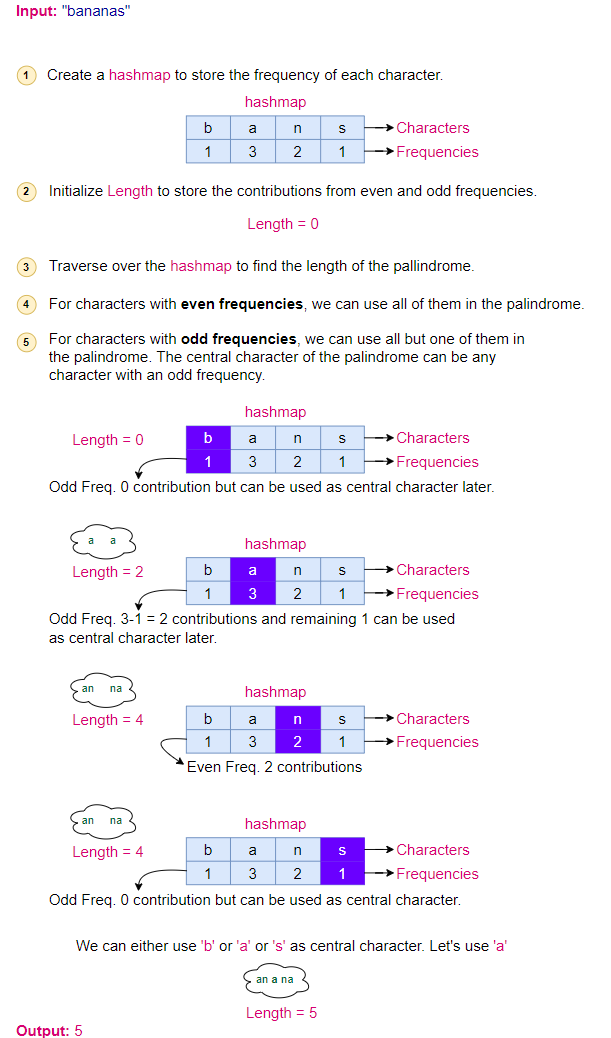
- For the string “bananas”, our hashmap will look like this:
- b: 1
- a: 3
- n: 2
- s: 1
- For the string “bananas”, our hashmap will look like this:
- Determine Palindrome Length:
- We’ll iterate through the hashmap to determine the length of the palindrome we can form.
- Even Frequencies:
- For characters with even frequencies, we can use all of them in the palindrome. For our string, the character ‘n’ has an even frequency.
- ‘n’ can contribute 2 characters.
- So far, we have a contribution of 2 characters to the palindrome.
- For characters with even frequencies, we can use all of them in the palindrome. For our string, the character ‘n’ has an even frequency.
- Odd Frequencies:
- For characters with odd frequencies, we can use all but one of them in the palindrome. The central character of the palindrome can be any character with an odd frequency.
- For our string, characters ‘b’, ‘a’, and ‘s’ have odd frequencies.
- ‘b’ can contribute 0 characters (leaving out 1).
- ‘a’ can contribute 2 characters (leaving out 1).
- ‘s’ can contribute 0 characters (leaving out 1).
- Additionally, one of the characters left out from the odd frequencies can be used as the central character of the palindrome. Let’s use ‘a’ for this purpose.
- So, from the odd frequencies, we have a contribution of 2 characters to the palindrome, plus 1 for the central character.
- Total Length:
- Combining the contributions from even and odd frequencies, we get a total palindrome length of 2 (from even frequencies) + 3 (from odd frequencies) = 5.
The longest palindrome that can be constructed from “bananas” is of length 5.
Here is the visual representation of the algorithm:
Code
Here is the code for this algorithm:
1 | class Solution: |
Time Complexity:
- Iterating through the string: We iterate through the entire string once to count the frequency of each character. This operation takes (O(n)) time, where (n) is the length of the string.
- Iterating through the hashmap: After counting the frequencies, we iterate through the hashmap to determine how many characters can be used to form the palindrome. In the worst case, this would be (O(26)) for the English alphabet, which is a constant time. However, in general terms, if we consider any possible character (not just English alphabet), this would be (O(k)), where (k) is the number of unique characters in the string. But since k <= n , this can also be considered (O(n)) in the worst case.
Combining the two steps, the overall time complexity is (O(n) + O(n) = O(n)).
Space Complexity:
Hashmap for character frequencies: The space taken by the hashmap is proportional to the number of unique characters in the string. In the worst case, this would be (O(26)) for the English alphabet, which is a constant space. However, in general terms, if we consider any possible character (not just English alphabet), this would be (O(k)), where (k) is the number of unique characters in the string. But since k <= n, this can also be considered (O(n)) in the worst case.
Thus, the space complexity of the algorithm is (O(n)).
Ransom Note (easy)
Top Interview 150 | 383. Ransom Note Design Gurus
Problem Statement
Given two strings, one representing a ransom note and the another representing the available letters from a magazine, determine if it’s possible to construct the ransom note using only the letters from the magazine. Each letter from the magazine can be used only once.
Examples:
- Example 1:
- Input: Ransom Note = “hello”, Magazine = “hellworld”
- Expected Output: true
- Justification: The word “hello” can be constructed from the letters in “hellworld”.
- Example 2:
- Input: Ransom Note = “notes”, Magazine = “stoned”
- Expected Output: true
- Justification: The word “notes” can be fully constructed from “stoned” from its first 5 letters.
- Example 3:
- Input: Ransom Note = “apple”, Magazine = “pale”
- Expected Output: false
- Justification: The word “apple” cannot be constructed from “pale” as we are missing one ‘p’.
Constraints:
- 1 <= ransomNote.length, magazine.length <= 10^5
- ransomNote and magazine consist of lowercase English letters.
Solution
To solve this problem, we will utilize a hashmap to keep track of the frequency of each character in the magazine. First, we iterate through the magazine, updating the hashmap with the count of each character. Then, we go through the ransom note. For each character in the note, we check if it exists in the hashmap and if its count is greater than zero. If it is, we decrease the count in the hashmap, indicating that we’ve used that letter. If at any point we find a character in the note that isn’t available in sufficient quantity in the magazine, we return false. If we successfully go through the entire note without this issue, we return true, indicating the note can be constructed from the magazine.
- Populate Frequency Map: Traverse the magazine string and populate a hashmap with the frequency of each character.
- Check Feasibility: Traverse the ransom note string. For each character, check its frequency in the hashmap. If the character is not present or its frequency is zero, return false. Otherwise, decrement the frequency of the character in the hashmap.
- Return Result: If we successfully traverse the ransom note without returning false, then it’s possible to construct the ransom note from the magazine. Return true.
Using a hashmap allows for efficient storage and retrieval of character frequencies, ensuring that we can determine the feasibility of constructing the ransom note in linear time.
Algorithm Walkthrough:
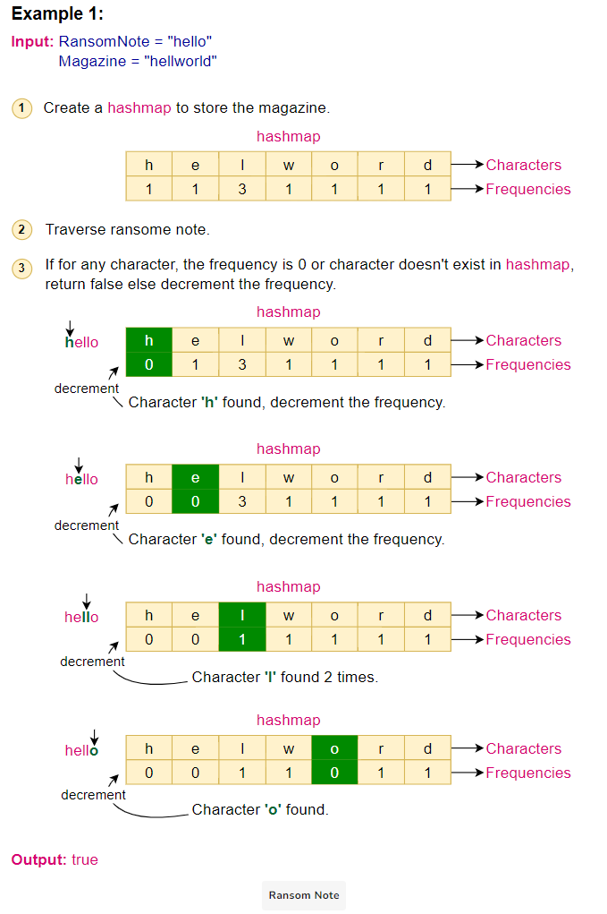
Given the ransom note “hello” and the magazine “hellworld”:
- Initialize an empty hashmap.
- Traverse the magazine “hellworld” and populate the hashmap with character frequencies: {‘h’:1, ‘e’:1, ‘l’:3, ‘w’:1, ‘o’:1, ‘r’:1, ‘d’:1}.
- Traverse the ransom note “hello”. For each character:
- Check its frequency in the hashmap.
- If the frequency is zero or the character is not present, return false.
- Otherwise, decrement the frequency of the character in the hashmap.
- Since we can traverse the entire ransom note without returning false, return true.
Here is the visual representation of the algorithm:
Code
Here is the code for this algorithm:
1 | from collections import defaultdict |
Complexity Analysis
Time Complexity: The algorithm traverses both the ransom note and the magazine once, making the time complexity O(n + m), where n is the length of the ransom note and m is the length of the magazine.
Space Complexity: The space complexity is determined by the hashmap, which in the worst case will have an entry for each unique character in the magazine. However, since the English alphabet has a fixed number of characters, the space complexity is O(1).